机器学习——决策树

决策树

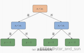
决策树可以理解为是一颗倒立的树，叶子在下端，根在最上面
一层一层连接的是交内部节点，内部节点主要是一些条件判断表达式，叶子叫叶节点，叶节点其实就是最终的预测结果，那么当输入x进去，一层一层的进行选择，就到最后的叶子节点，就完成整个流程，叶子节点的值就是最终的值。
决策树经常用来做分类任务，下面是基本的决策树的结构

决策树的构造

在构造决策树的时候需要尽可能的减少模型的复杂度，可见决策树的层数和节点数不要过多才最好。
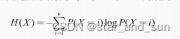
x,y的取值范围是1，。。。，n 则信息熵的公式

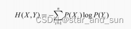
交叉熵

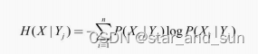
条件熵

信息增益

                         **i=h(x)-h(x|y)**

信息增益率

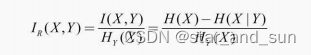
其中

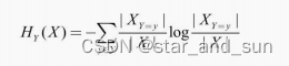
采用信息增益率可以减少模型整体的复杂度。
id3和c4.5
id3算法是基于信息增益来做的，c4.5是结合信息增益率来做的，只能解决分类问题。

cart算法
id3算法，c4.5只能解决分类问题。在回归问题中，采用cart算法，其采用了误差的平方作为标准

此外cart算法可以解决分类问题

import numpy as np
import matplotlib.pyplot as plt
import pandas as pd

# 读取数据
data = pd.read_csv('titanic/train.csv')
# 查看数据集信息和前5行具体内容，其中nan代表数据缺失
print(data.info())
print(data[:5])

# 删去编号、姓名、船票编号3列
data.drop(columns=['passengerid', 'name', 'ticket'], inplace=true)
#%%
feat_ranges = {}
cont_feat = ['age', 'fare'] # 连续特征
bins = 10 # 分类点数

for feat in cont_feat:
    # 数据集中存在缺省值nan，需要用np.nanmin和np.nanmax
    min_val = np.nanmin(data[feat]) 
    max_val = np.nanmax(data[feat])
    feat_ranges[feat] = np.linspace(min_val, max_val, bins).tolist()
    print(feat, '：') # 查看分类点
    for spt in feat_ranges[feat]:
        print(f'{spt:.4f}')
#%%
# 只有有限取值的离散特征
cat_feat = ['sex', 'pclass', 'sibsp', 'parch', 'cabin', 'embarked'] 
for feat in cat_feat:
    data[feat] = data[feat].astype('category') # 数据格式转为分类格式
    print(f'{feat}：{data[feat].cat.categories}') # 查看类别
    data[feat] = data[feat].cat.codes.to_list() # 将类别按顺序转换为整数
    ranges = list(set(data[feat]))
    ranges.sort()
    feat_ranges[feat] = ranges
#%%
# 将所有缺省值替换为-1
data.fillna(-1, inplace=true)
for feat in feat_ranges.keys():
    feat_ranges[feat] = [-1] + feat_ranges[feat]
#%%
# 划分训练集与测试集
np.random.seed(0)
feat_names = data.columns[1:]
label_name = data.columns[0]
# 重排下标之后，按新的下标索引数据
data = data.reindex(np.random.permutation(data.index))
ratio = 0.8
split = int(ratio * len(data))
train_x = data[:split].drop(columns=['survived']).to_numpy()
train_y = data['survived'][:split].to_numpy()
test_x = data[split:].drop(columns=['survived']).to_numpy()
test_y = data['survived'][split:].to_numpy()
print('训练集大小：', len(train_x))
print('测试集大小：', len(test_x))
print('特征数：', train_x.shape[1])
#%%
class node:

    def __init__(self):
        # 内部结点的feat表示用来分类的特征编号，其数字与数据中的顺序对应
        # 叶结点的feat表示该结点对应的分类结果
        self.feat = none
        # 分类值列表，表示按照其中的值向子结点分类
        self.split = none
        # 子结点列表，叶结点的child为空
        self.child = []
#%%
class decisiontree:

    def __init__(self, x, y, feat_ranges, lbd):
        self.root = node()
        self.x = x
        self.y = y
        self.feat_ranges = feat_ranges # 特征取值范围
        self.lbd = lbd # 正则化系数
        self.eps = 1e-8 # 防止数学错误log(0)和除以0
        self.t = 0 # 记录叶结点个数
        self.id3(self.root, self.x, self.y)

    # 工具函数，计算 a * log a
    def aloga(self, a):
        return a * np.log2(a + self.eps)

    # 计算某个子数据集的熵
    def entropy(self, y):
        cnt = np.unique(y, return_counts=true)[1] # 统计每个类别出现的次数
        n = len(y)
        ent = -np.sum([self.aloga(ni / n) for ni in cnt])
        return ent

    # 计算用feat <= val划分数据集的信息增益
    def info_gain(self, x, y, feat, val):
        # 划分前的熵
        n = len(y)
        if n == 0:
            return 0
        hx = self.entropy(y)
        hxy = 0 # h(x|y)
        # 分别计算h(x|x_f<=val)和h(x|x_f>val)
        y_l = y[x[:, feat] <= val]
        hxy += len(y_l) / len(y) * self.entropy(y_l)
        y_r = y[x[:, feat] > val]
        hxy += len(y_r) / len(y) * self.entropy(y_r)
        return hx - hxy

    # 计算特征feat <= val本身的复杂度h_y(x)
    def entropy_yx(self, x, y, feat, val):
        hyx = 0
        n = len(y)
        if n == 0:
            return 0
        y_l = y[x[:, feat] <= val]
        hyx += -self.aloga(len(y_l) / n)
        y_r = y[x[:, feat] > val]
        hyx += -self.aloga(len(y_r) / n)
        return hyx

    # 计算用feat <= val划分数据集的信息增益率
    def info_gain_ratio(self, x, y, feat, val):
        ig = self.info_gain(x, y, feat, val)
        hyx = self.entropy_yx(x, y, feat, val)
        return ig / hyx

    # 用id3算法递归分裂结点，构造决策树
    def id3(self, node, x, y):
        # 判断是否已经分类完成
        if len(np.unique(y)) == 1:
            node.feat = y[0]
            self.t += 1
            return
        
        # 寻找最优分类特征和分类点
        best_igr = 0
        best_feat = none
        best_val = none
        for feat in range(len(feat_names)):
            for val in self.feat_ranges[feat_names[feat]]:
                igr = self.info_gain_ratio(x, y, feat, val)
                if igr > best_igr:
                    best_igr = igr
                    best_feat = feat
                    best_val = val
        
        # 计算用best_feat <= best_val分类带来的代价函数变化
        # 由于分裂叶结点只涉及该局部，我们只需要计算分裂前后该结点的代价函数
        # 当前代价
        cur_cost = len(y) * self.entropy(y) + self.lbd
        # 分裂后的代价，按best_feat的取值分类统计
        # 如果best_feat为none，说明最优的信息增益率为0，
        # 再分类也无法增加信息了，因此将new_cost设置为无穷大
        if best_feat is none:
            new_cost = np.inf
        else:
            new_cost = 0
            x_feat = x[:, best_feat]
            # 获取划分后的两部分，计算新的熵
            new_y_l = y[x_feat <= best_val]
            new_cost += len(new_y_l) * self.entropy(new_y_l)
            new_y_r = y[x_feat > best_val]
            new_cost += len(new_y_r) * self.entropy(new_y_r)
            # 分裂后会有两个叶结点
            new_cost += 2 * self.lbd

        if new_cost <= cur_cost:
            # 如果分裂后代价更小，那么执行分裂
            node.feat = best_feat
            node.split = best_val
            l_child = node()
            l_x = x[x_feat <= best_val]
            l_y = y[x_feat <= best_val]
            self.id3(l_child, l_x, l_y)
            r_child = node()
            r_x = x[x_feat > best_val]
            r_y = y[x_feat > best_val]
            self.id3(r_child, r_x, r_y)
            node.child = [l_child, r_child]
        else:
            # 否则将当前结点上最多的类别作为该结点的类别
            vals, cnt = np.unique(y, return_counts=true)
            node.feat = vals[np.argmax(cnt)]
            self.t += 1

    # 预测新样本的分类
    def predict(self, x):
        node = self.root
        # 从根结点开始向下寻找，到叶结点结束
        while node.split is not none:
            # 判断x应该处于哪个子结点
            if x[node.feat] <= node.split:
                node = node.child[0]
            else:
                node = node.child[1]
        # 到达叶结点，返回类别
        return node.feat

    # 计算在样本x，标签y上的准确率
    def accuracy(self, x, y):
        correct = 0
        for x, y in zip(x, y):
            pred = self.predict(x)
            if pred == y:
                correct += 1
        return correct / len(y)
#%%
dt = decisiontree(train_x, train_y, feat_ranges, lbd=1.0)
print('叶结点数量：', dt.t)

# 计算在训练集和测试集上的准确率
print('训练集准确率：', dt.accuracy(train_x, train_y))
print('测试集准确率：', dt.accuracy(test_x, test_y))
#%%
from sklearn import tree

# criterion表示分类依据，max_depth表示树的最大深度
# entropy生成的是c4.5分类树
c45 = tree.decisiontreeclassifier(criterion='entropy', max_depth=6)
c45.fit(train_x, train_y)
# gini生成的是cart分类树
cart = tree.decisiontreeclassifier(criterion='gini', max_depth=6)
cart.fit(train_x, train_y)

c45_train_pred = c45.predict(train_x)
c45_test_pred = c45.predict(test_x)
cart_train_pred = cart.predict(train_x)
cart_test_pred = cart.predict(test_x)
print(f'训练集准确率：c4.5：{np.mean(c45_train_pred == train_y)}，' \
    f'cart：{np.mean(cart_train_pred == train_y)}')
print(f'测试集准确率：c4.5：{np.mean(c45_test_pred == test_y)}，' \
    f'cart：{np.mean(cart_test_pred == test_y)}')
#%%
!pip install pydotplus

from six import stringio
import pydotplus

dot_data = stringio()
tree.export_graphviz( # 导出sklearn的决策树的可视化数据
    c45,
    out_file=dot_data,
    feature_names=feat_names,
    class_names=['non-survival', 'survival'],
    filled=true, 
    rounded=true,
    impurity=false
)
# 用pydotplus生成图像
graph = pydotplus.graph_from_dot_data(
    dot_data.getvalue().replace('\n', '')) 
graph.write_png('tree.png')