【计算机视觉】Gaussian Splatting源码解读补充（二）

本文是对学习笔记之——3d gaussian splatting源码解读的补充，并订正了一些错误。

---

三、相机相关

scene/cameras.py：class camera

class camera(nn.module):
    def __init__(self, colmap_id, r, t, fovx, fovy, image, gt_alpha_mask,
                 image_name, uid,
                 trans=np.array([0.0, 0.0, 0.0]), scale=1.0, data_device = "cuda"
                 ):
        super(camera, self).__init__()

        self.uid = uid
        self.colmap_id = colmap_id
        self.r = r # 旋转矩阵
        self.t = t # 平移向量
        self.fovx = fovx # x方向视场角
        self.fovy = fovy # y方向视场角
        self.image_name = image_name

        try:
            self.data_device = torch.device(data_device)
        except exception as e:
            print(e)
            print(f"[warning] custom device {data_device} failed, fallback to default cuda device" )
            self.data_device = torch.device("cuda")

        self.original_image = image.clamp(0.0, 1.0).to(self.data_device) # 原始图像
        self.image_width = self.original_image.shape[2] # 图像宽度
        self.image_height = self.original_image.shape[1] # 图像高度

        if gt_alpha_mask is not none:
            self.original_image *= gt_alpha_mask.to(self.data_device)
        else:
            self.original_image *= torch.ones((1, self.image_height, self.image_width), device=self.data_device)

		# 距离相机平面znear和zfar之间且在视锥内的物体才会被渲染
        self.zfar = 100.0 # 最远能看到多远
        self.znear = 0.01 # 最近能看到多近

        self.trans = trans # 相机中心的平移
        self.scale = scale # 相机中心坐标的缩放

        self.world_view_transform = torch.tensor(getworld2view2(r, t, trans, scale)).transpose(0, 1).cuda() # 世界到相机坐标系的变换矩阵，4×4
        self.projection_matrix = getprojectionmatrix(znear=self.znear, zfar=self.zfar, fovx=self.fovx, fovy=self.fovy).transpose(0,1).cuda() # 投影矩阵
        self.full_proj_transform = (self.world_view_transform.unsqueeze(0).bmm(self.projection_matrix.unsqueeze(0))).squeeze(0) # 从世界坐标系到图像的变换矩阵
        self.camera_center = self.world_view_transform.inverse()[3, :3] # 相机在世界坐标系下的坐标

其中出现的辅助函数：

# utils/graphic_utils.py
def getworld2view2(r, t, translate=np.array([.0, .0, .0]), scale=1.0):
    rt = np.zeros((4, 4)) # 按理来说是世界到相机的变换矩阵，但没有加平移和缩放
    rt[:3, :3] = r.transpose()
    rt[:3, 3] = t
    rt[3, 3] = 1.0

    c2w = np.linalg.inv(rt) # 相机到世界的变换矩阵
    cam_center = c2w[:3, 3] # 相机中心在世界中的坐标，即c2w矩阵第四列的三维平移向量
    cam_center = (cam_center + translate) * scale # 相机中心坐标需要平移和缩放处理
    c2w[:3, 3] = cam_center # 重新填入c2w矩阵
    rt = np.linalg.inv(c2w) # 再取逆获得w2c矩阵
    return np.float32(rt)

四、前向传播（渲染）：submodules/diff-gaussian-rasterization/cuda_rasterizer/forward.cu

预备知识：cuda编程基础

这部分的参考资料：

[1] cuda tutorial
[2] an even easier introduction to cuda
[3] introduction to cuda programming

cuda是一个为支持cuda的gpu提供的平台和编程模型。该平台使gpu能够进行通用计算。cuda提供了c/c++语言扩展和api，以便用户利用gpu进行高效计算。一般称cpu为host，gpu为device。

cuda c++语言中有一个加在函数前面的关键字__global__，用于表明该函数是运行在gpu上的，并且可以被cpu调用。这种函数称为kernel。

当我们调用kernel的时候，需要在函数名和括号之间加上<<<m, t>>>，其中m是block的个数，t是每个block中线程的个数。这些线程都是并行执行的，每个线程中都在执行该函数。

根据参考资料[3]，gpu在同一时刻运行一个kernel（也就是一组任务），kernel运行在grid上，每个grid由多个block组成（他们是独立的alu组），每个block有多个线程。

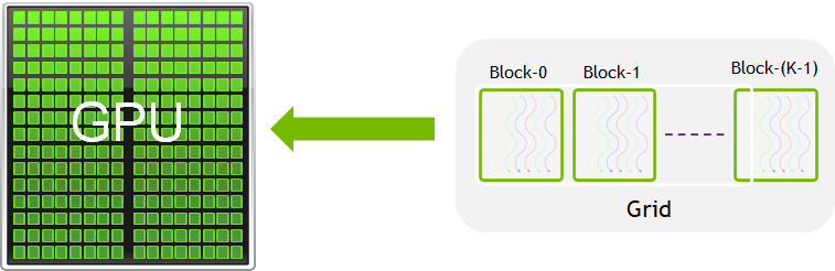
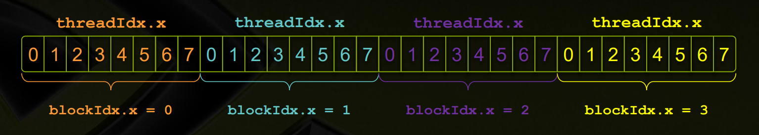
同一block中的线程一般合作完成任务，它们可以共享内存（这部分内存速度极快，用__shared__关键字声明）。每个线程“知道”它在哪个block（通过访问内置变量blockidx.x）和它是第几个线程（通过访问变量threadidx.x），以及每个block有多少个线程（blockdim.x），从而确定它应该完成什么任务。实际上线程和block的索引是三维的，这里只举了一个一维的例子。

注意gpu和cpu的内存是隔离的，想要操作显存或者在显存和cpu内存之间进行交流必须显示的声明这些操作。指针也是不一样的，有可能虽然都是int*，但表示的含义却不同：device指针指向显存，host指针指向cpu内存。cuda提供了操作内存的内置函数：cudamalloc、cudafree、cudamemcpy等，它们分别类似于c函数malloc、free和memcpy。

关于同步方面，内置函数 __syncthreads()可以同步一个block中的所有线程。在cpu中调用内置函数cudadevicesynchronize()可以可以阻塞cpu，直到所有先前发出的cuda调用都完成为止。

另外还有__host__关键字和__device__关键字，前者表示该函数只编译成cpu版本（这是默认状态），后者表示只编译成gpu版本。二者同时使用表示编译cpu和gpu两个版本。从cpu调用__device__函数和从gpu调用__host__函数都会报错。

以下是一个cuda并行计算向量加法的示例：

#include <stdio.h>

int a[10] = {0, 1, 2, 3, 4, 5, 6, 7, 8, 9};
int b[10] = {0, 10, 20, 30, 40, 50, 60, 70, 80, 90};
int c[10];

__global__ void vec_add(int* a, int* b, int* c)
{
    int i = blockidx.x * blockdim.x + threadidx.x;
    c[i] = a[i] + b[i];
}

int main()
{
    int* gpua, *gpub, *gpuc;
    int sz = 10 * sizeof(int);
    cudamalloc((void**)&gpua, sz); // 在gpu中分配内存
    cudamalloc((void**)&gpub, sz);
    cudamalloc((void**)&gpuc, sz);
    cudamemcpy(gpua, a, sz, cudamemcpyhosttodevice); // 拷贝cpu中的数组到gpu
    cudamemcpy(gpub, b, sz, cudamemcpyhosttodevice);
    vec_add<<<2, 5>>>(gpua, gpub, gpuc); // 调用kernel
    cudadevicesynchronize(); // 等gpu执行完（这里其实不是很有必要）
    cudamemcpy(c, gpuc, sz, cudamemcpydevicetohost); // 把gpu的计算结果拷贝到cpu
    for(int i = 0; i < 10; i++)
    {
        printf("%d\n", c[i]); // 输出结果，结果为0、11、22、……、99
    }
    return 0;
}

有了这些预备知识之后，我们就可以开始看代码了。在看cuda代码之前，我们先看看gaussian_renderer/__init__.py中的render函数。

def render(viewpoint_camera, pc : gaussianmodel, pipe, bg_color : torch.tensor, scaling_modifier = 1.0, override_color = none)

def render(viewpoint_camera, pc : gaussianmodel, pipe, bg_color : torch.tensor, scaling_modifier = 1.0, override_color = none):
	'''
	viewpoint_camera: scene.cameras.camera类的实例
	pipe: 流水线，规定了要干什么
	'''
    # create zero tensor. we will use it to make pytorch return gradients of the 2d (screen-space) means
    screenspace_points = torch.zeros_like(pc.get_xyz, dtype=pc.get_xyz.dtype, requires_grad=true, device="cuda") + 0
    try:
        screenspace_points.retain_grad() # 让screenspace_points在反向传播时接受梯度
    except:
        pass

    # set up rasterization configuration
    tanfovx = math.tan(viewpoint_camera.fovx * 0.5)
    tanfovy = math.tan(viewpoint_camera.fovy * 0.5)

    raster_settings = gaussianrasterizationsettings(
        image_height=int(viewpoint_camera.image_height),
        image_width=int(viewpoint_camera.image_width),
        tanfovx=tanfovx,
        tanfovy=tanfovy,
        bg=bg_color, # 背景颜色
        scale_modifier=scaling_modifier,
        viewmatrix=viewpoint_camera.world_view_transform, # w2c矩阵
        projmatrix=viewpoint_camera.full_proj_transform, # 世界到图像的投影矩阵
        sh_degree=pc.active_sh_degree, # 目前的球谐阶数
        campos=viewpoint_camera.camera_center, # camera center position，相机中心文职
        prefiltered=false,
        debug=pipe.debug
    )

    rasterizer = gaussianrasterizer(raster_settings=raster_settings)

    means3d = pc.get_xyz
    means2d = screenspace_points # 疑似各个gaussian的中心投影到在图像中的坐标
    opacity = pc.get_opacity # 不透明度

    # if precomputed 3d covariance is provided, use it. if not, then it will be computed from
    # scaling / rotation by the rasterizer.
    scales = none
    rotations = none
    cov3d_precomp = none
    if pipe.compute_cov3d_python:
        cov3d_precomp = pc.get_covariance(scaling_modifier)
    else:
        scales = pc.get_scaling
        rotations = pc.get_rotation

    # if precomputed colors are provided, use them. otherwise, if it is desired to precompute colors
    # from shs in python, do it. if not, then sh -> rgb conversion will be done by rasterizer.
    shs = none
    colors_precomp = none
    if override_color is none:
        if pipe.convert_shs_python:
            shs_view = pc.get_features.transpose(1, 2).view(-1, 3, (pc.max_sh_degree+1)**2)
            dir_pp = (pc.get_xyz - viewpoint_camera.camera_center.repeat(pc.get_features.shape[0], 1))
            dir_pp_normalized = dir_pp/dir_pp.norm(dim=1, keepdim=true)
            	# 找到高斯中心到相机的光线在单位球体上的坐标
            sh2rgb = eval_sh(pc.active_sh_degree, shs_view, dir_pp_normalized)
            	# 球谐的傅里叶系数转成rgb颜色
            colors_precomp = torch.clamp_min(sh2rgb + 0.5, 0.0)
        else:
            shs = pc.get_features
    else:
        colors_precomp = override_color

    # rasterize visible gaussians to image, obtain their radii (on screen). 
    rendered_image, radii = rasterizer(
        means3d = means3d,
        means2d = means2d,
        shs = shs,
        colors_precomp = colors_precomp,
        opacities = opacity,
        scales = scales,
        rotations = rotations,
        cov3d_precomp = cov3d_precomp)

    # those gaussians that were frustum culled or had a radius of 0 were not visible.
    # they will be excluded from value updates used in the splitting criteria.
    return {"render": rendered_image,
            "viewspace_points": screenspace_points,
            "visibility_filter" : radii > 0,
            "radii": radii}

cuda文件rasterizer_impl.cu: submodules/diff-gaussian-rasterization/cuda_rasterizer

1. 引用头文件

#include "rasterizer_impl.h"
#include <iostream>
#include <fstream>
#include <algorithm>
#include <numeric>
#include <cuda.h>
#include "cuda_runtime.h"
#include "device_launch_parameters.h"
#include <cub/cub.cuh> // cuda的cub库
#include <cub/device/device_radix_sort.cuh>
#define glm_force_cuda
#include <glm/glm.hpp> // glm (opengl mathematics)库

#include <cooperative_groups.h> // cuda 9引入的cooperative groups库
#include <cooperative_groups/reduce.h>
namespace cg = cooperative_groups;

#include "auxiliary.h"
#include "forward.h"
#include "backward.h"

有一些库需要我们讲解一下。

(1) cooperative groups

参考资料：

• cooperative groups: flexible cuda thread programming
  
• 这个库的官方文档

我们直到 __syncthreads()函数提供了在一个block内同步各线程的方法，但有时要同步block内的一部分线程或者多个block的线程，这时候就需要cooperative groups库了。这个库定义了划分和同步一组线程的方法。

在gaussian splatting的所有cuda代码中，这个库仅以两种方式被调用：

🥕(a)

auto idx = cg::this_grid().thread_rank();

cg::this_grid()返回一个cg::grid_group实例，表示当前线程所处的grid。他有一个方法thread_rank()返回当前线程在该grid中排第几。

🥕(b)

auto block = cg::this_thread_block();

cg::this_thread_block返回一个cg::thread_block实例。代码中用到的成员函数有：

• block.sync()：同步该block中的所有线程（等价于__syncthreads()）。
• block.thread_rank()：返回非负整数，表示当前线程在该block中排第几。
• block.group_index()：返回一个cg::dim3实例，表示该block在grid中的三维索引。
• block.thread_index()：返回一个cg::dim3实例，表示当前线程在block中的三维索引。

(2) cub

参考资料：cub api

换言之，cub就是针对不同的计算等级：线程、wap、block、device等设计了并行算法。例如，reduce函数有四个版本：threadreduce、warpreduce、blockreduce、devicereduce。

diff-gaussian-rasterization模块调用了cub库的两个函数：

⭐️ (a) cub::devicescan::inclusivesum

这个函数是算前缀和的。所谓"inclusive"就是第$i$个数被计入第$i$个和中。函数定义如下：

template<typename inputiteratort, typename outputiteratort>
static inline cudaerror_t inclusivesum(
	void *d_temp_storage, // 额外需要的临时显存空间
	size_t &temp_storage_bytes, // 临时显存空间的大小
	inputiteratort d_in, // 输入指针
	outputiteratort d_out, // 输出指针
	int num_items, // 元素个数
	cudastream_t stream = 0)

⭐️ (b) cub::deviceradixsort::sortpairs：device级别的并行基数排序

该函数根据key将(key, value)对进行升序排序。这是一种稳定排序。

函数定义如下：

template<typename keyt, typename valuet, typename numitemst>
static inline cudaerror_t sortpairs(
	void *d_temp_storage, // 排序时用到的临时显存空间
	size_t &temp_storage_bytes, // 临时显存空间的大小
	const keyt *d_keys_in,         keyt *d_keys_out, // key的输入和输出指针
	const valuet *d_values_in,     valuet *d_values_out, // value的输入和输出指针
	numitemst num_items, // 对多少个条目进行排序
	int begin_bit = 0, // 低位
	int end_bit = sizeof(keyt) * 8, // 高位
	cudastream_t stream = 0)
	// 按照[begin_bit, end_bit)内的位进行排序

示例代码：

#include <stdio.h>
#include <cub/cub.cuh>
// or equivalently <cub/device/device_radix_sort.cuh>

int main()
{
    // declare, allocate, and initialize device-accessible pointers
    // for sorting data
    int  num_items = 7;
    int  keys_in[7] = {8, 6, 7, 5, 3, 0, 9};
    int* d_keys_in, *d_keys_out;
    int  values_in[7] = {0, 1, 2, 3, 4, 5, 6};
    int* d_values_in, *d_values_out;

    int keys_out[7], values_out[7];

    // 下面把数据搬到显存中
    int sz = 7 * sizeof(int);
    cudamalloc((void**)&d_values_in, sz);
    cudamalloc((void**)&d_values_out, sz);
    cudamalloc((void**)&d_keys_in, sz);
    cudamalloc((void**)&d_keys_out, sz);
    cudamemcpy(d_keys_in, keys_in, sz, cudamemcpyhosttodevice);
    cudamemcpy(d_values_in, values_in, sz, cudamemcpyhosttodevice);

    // determine temporary device storage requirements
    void     *d_temp_storage = null;
    size_t   temp_storage_bytes = 0;
    cub::deviceradixsort::sortpairs(d_temp_storage, temp_storage_bytes,
        d_keys_in, d_keys_out, d_values_in, d_values_out, num_items);

    // allocate temporary storage
    cudamalloc(&d_temp_storage, temp_storage_bytes);

    // run sorting operation
    cub::deviceradixsort::sortpairs(d_temp_storage, temp_storage_bytes,
        d_keys_in, d_keys_out, d_values_in, d_values_out, num_items);

    // 结果：
    // d_keys_out            <-- [0, 3, 5, 6, 7, 8, 9]
    // d_values_out          <-- [5, 4, 3, 1, 2, 0, 6]

    // 把算好的数据搬回来
    cudamemcpy(keys_out, d_keys_out, sz, cudamemcpydevicetohost);
    cudamemcpy(values_out, d_values_out, sz, cudamemcpydevicetohost);

    puts("keys");
    for(int i = 0; i < 7; i++)
    {
        printf("%d ", keys_out[i]);
    }
    puts("\nvalues");
    for(int i = 0; i < 7; i++)
    {
        printf("%d ", values_out[i]);
    }

    cudafree(d_keys_in);
    cudafree(d_keys_out);
    cudafree(d_values_in);
    cudafree(d_values_out);

    return 0;
}

(3) glm

参考资料：glm的github页面

glm意为“opengl mathematics”，是一个专为图形学设计的只有头文件的c++数学库。

gaussian splatting的代码中用到了glm::vec3（三维向量）, glm::vec4（四维向量）, glm::mat3（3×3矩阵）和glm::dot（向量点积）。

2. gethighermsb

// helper function to find the next-highest bit of the msb
// on the cpu.
uint32_t gethighermsb(uint32_t n)
{
	uint32_t msb = sizeof(n) * 4;
	uint32_t step = msb;
	while (step > 1)
	{
		step /= 2;
		if (n >> msb)
			msb += step;
		else
			msb -= step;
	}
	if (n >> msb)
		msb++;
	return msb;
}

这个函数似乎是用二分法检测n表示成二进制数除去前导零有几位（n=0时返回1）。我写了一个测试程序推测它的功能：

#include <iostream>
uint32_t gethighermsb(uint32_t n);

int main()
{
    uint32_t n[] = {0b0, 0b1, 0b10, 0b11, 0b111, 0b10101, 0b1110001};
    for(int i = 0; i < sizeof(n) / sizeof(uint32_t); i++)
        std::cout << gethighermsb(n[i]) << ", ";
    // 结果：1, 1, 2, 2, 3, 5, 7,
}

该函数只被调用过一次（在cudarasterizer::rasterizer::forward函数中），我们随后再推断它的具体含义。

3. checkfrustum和markvisible

根据函数命名和上下文推断，这两个函数的作用是检查一些gaussians是否在一个给定相机的视锥内，从而确定它能不能被该相机看见。

// wrapper method to call auxiliary coarse frustum containment test.
// mark all gaussians that pass it.
__global__ void checkfrustum(int p, // 需要检查的点的个数
	const float* orig_points, // 需要检查的点的世界坐标
	const float* viewmatrix, // w2c矩阵
	const float* projmatrix, // 投影矩阵
	bool* present) // 返回值，表示能不能被看见
{
	auto idx = cg::this_grid().thread_rank();
	if (idx >= p)
		return;

	float3 p_view;
	present[idx] = in_frustum(idx, orig_points, viewmatrix, projmatrix, false, p_view);
}

// mark gaussians as visible/invisible, based on view frustum testing
void cudarasterizer::rasterizer::markvisible(
	int p,
	float* means3d, // gaussians的中心点坐标
	float* viewmatrix,
	float* projmatrix,
	bool* present)
{
	checkfrustum << <(p + 255) / 256, 256 >> > (
		p,
		means3d,
		viewmatrix, projmatrix,
		present);
}

4. 几个fromchunk

这些函数的作用是从以char数组形式存储的二进制块中读取geometrystate、imagestate、binningstate等类的信息。

cudarasterizer::geometrystate cudarasterizer::geometrystate::fromchunk(char*& chunk, size_t p)
{
	geometrystate geom;
	obtain(chunk, geom.depths, p, 128);
	obtain(chunk, geom.clamped, p * 3, 128);
	obtain(chunk, geom.internal_radii, p, 128);
	obtain(chunk, geom.means2d, p, 128);
	obtain(chunk, geom.cov3d, p * 6, 128);
	obtain(chunk, geom.conic_opacity, p, 128);
	obtain(chunk, geom.rgb, p * 3, 128);
	obtain(chunk, geom.tiles_touched, p, 128);
	cub::devicescan::inclusivesum(nullptr, geom.scan_size, geom.tiles_touched, geom.tiles_touched, p);
	obtain(chunk, geom.scanning_space, geom.scan_size, 128);
	obtain(chunk, geom.point_offsets, p, 128);
	return geom;
}

cudarasterizer::imagestate cudarasterizer::imagestate::fromchunk(char*& chunk, size_t n)
{
	imagestate img;
	obtain(chunk, img.accum_alpha, n, 128);
	obtain(chunk, img.n_contrib, n, 128);
	obtain(chunk, img.ranges, n, 128);
	return img;
}

cudarasterizer::binningstate cudarasterizer::binningstate::fromchunk(char*& chunk, size_t p)
{
	binningstate binning;
	obtain(chunk, binning.point_list, p, 128);
	obtain(chunk, binning.point_list_unsorted, p, 128);
	obtain(chunk, binning.point_list_keys, p, 128);
	obtain(chunk, binning.point_list_keys_unsorted, p, 128);
	cub::deviceradixsort::sortpairs(
		nullptr, binning.sorting_size,
		binning.point_list_keys_unsorted, binning.point_list_keys,
		binning.point_list_unsorted, binning.point_list, p);
	obtain(chunk, binning.list_sorting_space, binning.sorting_size, 128);
	return binning;
}

5. 为排序做准备：duplicatewithkeys

// generates one key/value pair for all gaussian / tile overlaps. 
// run once per gaussian (1:n mapping).
__global__ void duplicatewithkeys(
	int p,
	const float2* points_xy,
	const float* depths,
	const uint32_t* offsets,
	uint64_t* gaussian_keys_unsorted,
	uint32_t* gaussian_values_unsorted,
	int* radii,
	dim3 grid)
{
	auto idx = cg::this_grid().thread_rank(); // 线程索引，该显线程处理第idx个gaussian
	if (idx >= p)
		return;

	// generate no key/value pair for invisible gaussians
	if (radii[idx] > 0)
	{
		// find this gaussian's offset in buffer for writing keys/values.
		uint32_t off = (idx == 0) ? 0 : offsets[idx - 1];
		uint2 rect_min, rect_max;

		getrect(points_xy[idx], radii[idx], rect_min, rect_max, grid);
			// 因为要给gaussian覆盖的每个tile生成一个(key, value)对，
			// 所以先获取它占了哪些tile

		// for each tile that the bounding rect overlaps, emit a 
		// key/value pair. the key is |  tile id  |      depth      |,
		// and the value is the id of the gaussian. sorting the values 
		// with this key yields gaussian ids in a list, such that they
		// are first sorted by tile and then by depth. 
		for (int y = rect_min.y; y < rect_max.y; y++)
		{
			for (int x = rect_min.x; x < rect_max.x; x++)
			{
				uint64_t key = y * grid.x + x; // tile的id
				key <<= 32; // 放在高位
				key |= *((uint32_t*)&depths[idx]); // 低位是深度
				gaussian_keys_unsorted[off] = key;
				gaussian_values_unsorted[off] = idx;
				off++; // 数组中的偏移量
			}
		}
	}
}

6. 排序之后的处理：identifytileranges

// check keys to see if it is at the start/end of one tile's range in 
// the full sorted list. if yes, write start/end of this tile. 
// run once per instanced (duplicated) gaussian id.
__global__ void identifytileranges(
	int l, // 排序列表中的元素个数
	uint64_t* point_list_keys, // 排过序的keys
	uint2* ranges)
		// ranges[tile_id].x和y表示第tile_id个tile在排过序的列表中的起始和终止地址
{
	auto idx = cg::this_grid().thread_rank();
	if (idx >= l)
		return;

	// read tile id from key. update start/end of tile range if at limit.
	uint64_t key = point_list_keys[idx];
	uint32_t currtile = key >> 32; // 当前tile
	if (idx == 0)
		ranges[currtile].x = 0; // 边界条件：tile 0的起始位置
	else
	{
		uint32_t prevtile = point_list_keys[idx - 1] >> 32;
		if (currtile != prevtile)
			// 上一个元素和我处于不同的tile，
			// 那我是上一个tile的终止位置和我所在tile的起始位置
		{
			ranges[prevtile].y = idx;
			ranges[currtile].x = idx;
		}
	}
	if (idx == l - 1)
		ranges[currtile].y = l; // 边界条件：最后一个tile的终止位置
}

7. 重头戏：前向传播forward

原文第6节（fast differentiable rasterizer for gaussians）：

附录c中的伪代码如下：

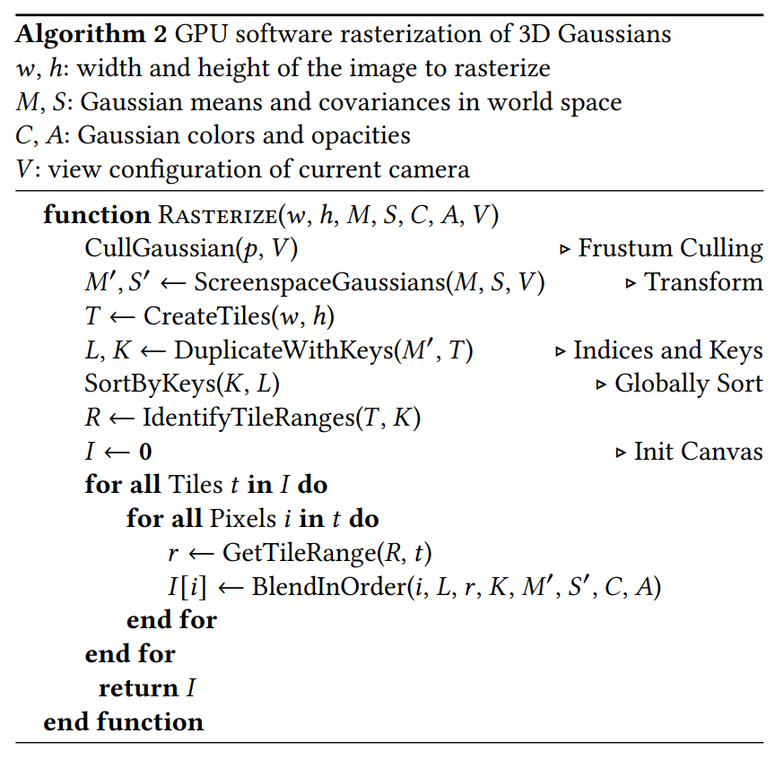
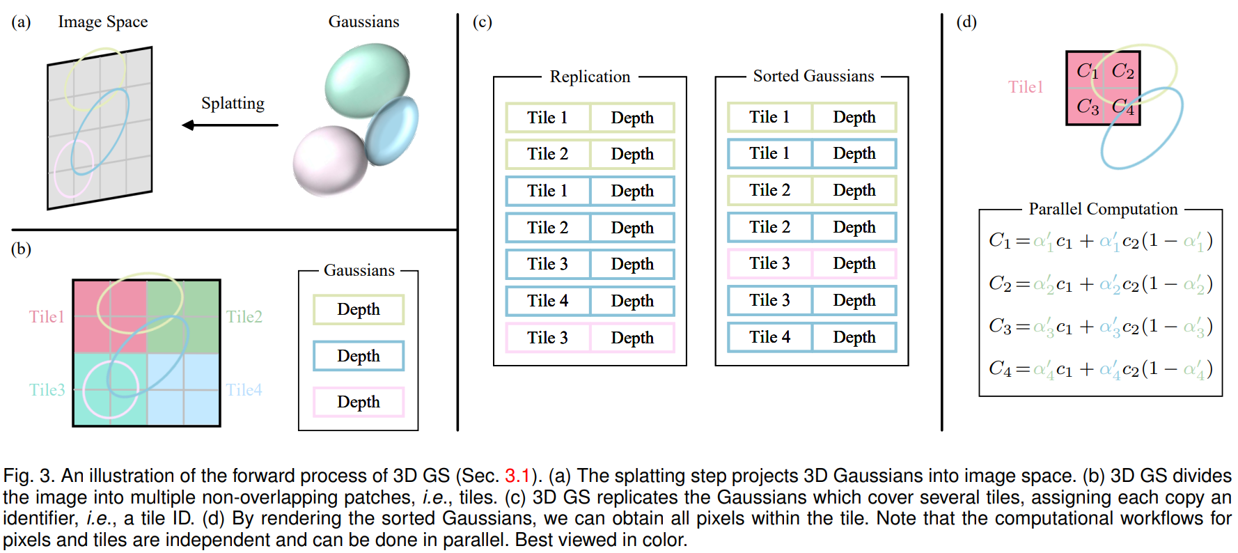
前向传播过程可以用该图片概括（出处：a survey on 3d gaussian splatting）：

// forward rendering procedure for differentiable rasterization
// of gaussians.
int cudarasterizer::rasterizer::forward(
	std::function<char* (size_t)> geometrybuffer,
	std::function<char* (size_t)> binningbuffer,
	std::function<char* (size_t)> imagebuffer,
	/*
		上面的三个参数是用于分配缓冲区的函数，
		在submodules/diff-gaussian-rasterization/rasterize_points.cu中定义
	*/
	const int p, // gaussian的数量
	int d, // 对应于gaussianmodel.active_sh_degree，是球谐度数（本文参考的学习笔记在这里是错误的）
	int m, // rgb三通道的球谐傅里叶系数个数，应等于3 × (d + 1)²（本文参考的学习笔记在这里也是错误的）
	const float* background,
	const int width, int height, // 图片宽高
	const float* means3d, // gaussians的中心坐标
	const float* shs, // 球谐系数
	const float* colors_precomp, // 预先计算的rgb颜色
	const float* opacities, // 不透明度
	const float* scales, // 缩放
	const float scale_modifier, // 缩放的修正项
	const float* rotations, // 旋转
	const float* cov3d_precomp, // 预先计算的3维协方差矩阵
	const float* viewmatrix, // w2c矩阵
	const float* projmatrix, // 投影矩阵
	const float* cam_pos, // 相机坐标
	const float tan_fovx, float tan_fovy, // 视场角一半的正切值
	const bool prefiltered,
	float* out_color, // 输出的颜色
	int* radii, // 各gaussian在像平面上用3σ原则截取后的半径
	bool debug)
{
	const float focal_y = height / (2.0f * tan_fovy); // y方向的焦距
	const float focal_x = width / (2.0f * tan_fovx); // x方向的焦距
	/*
		注意tan_fov = tan(fov / 2) （见上面的render函数）。
		而tan(fov / 2)就是图像宽/高的一半与焦距之比。
		以x方向为例，tan(fovx / 2) = width / 2 / focal_x，
		故focal_x = width / (2 * tan(fovx / 2)) = width / (2 * tan_fovx)。
	*/

	// 下面初始化一些缓冲区
	size_t chunk_size = required<geometrystate>(p); // geometrystate占据空间的大小
	char* chunkptr = geometrybuffer(chunk_size);
	geometrystate geomstate = geometrystate::fromchunk(chunkptr, p);

	if (radii == nullptr)
	{
		radii = geomstate.internal_radii;
	}

	dim3 tile_grid((width + block_x - 1) / block_x, (height + block_y - 1) / block_y, 1);
		// block_x = block_y = 16，准备分解成16×16的tiles。
		// 之所以不能分解成更大的tiles，是因为对于同一张图片的离得较远的像素点而言
		// gaussian按深度排序的结果可能是不同的。
		// （想象一下两个gaussians离像平面很近，一个靠近图像左边缘，一个靠近右边缘）
		// dim3是cuda定义的含义x,y,z三个成员的三维unsigned int向量类。
		// tile_grid就是x和y方向上tile的个数。
	dim3 block(block_x, block_y, 1);

	// dynamically resize image-based auxiliary buffers during training
	size_t img_chunk_size = required<imagestate>(width * height);
	char* img_chunkptr = imagebuffer(img_chunk_size);
	imagestate imgstate = imagestate::fromchunk(img_chunkptr, width * height);

	if (num_channels != 3 && colors_precomp == nullptr)
	{
		throw std::runtime_error("for non-rgb, provide precomputed gaussian colors!");
	}

	// run preprocessing per-gaussian (transformation, bounding, conversion of shs to rgb)
	check_cuda(forward::preprocess(
		p, d, m,
		means3d,
		(glm::vec3*)scales,
		scale_modifier,
		(glm::vec4*)rotations,
		opacities,
		shs,
		geomstate.clamped,
		cov3d_precomp,
		colors_precomp,
		viewmatrix, projmatrix,
		(glm::vec3*)cam_pos,
		width, height,
		focal_x, focal_y,
		tan_fovx, tan_fovy,
		radii,
		geomstate.means2d, // gaussian投影到像平面上的中心坐标
		geomstate.depths, // gaussian的深度
		geomstate.cov3d, // 三维协方差矩阵
		geomstate.rgb, // 颜色
		geomstate.conic_opacity, // 椭圆二次型的矩阵和不透明度的打包向量
		tile_grid, // 
		geomstate.tiles_touched,
		prefiltered
	), debug) // 预处理，主要涉及把3d的gaussian投影到2d

	// compute prefix sum over full list of touched tile counts by gaussians
	// e.g., [2, 3, 0, 2, 1] -> [2, 5, 5, 7, 8]
	check_cuda(cub::devicescan::inclusivesum(geomstate.scanning_space, geomstate.scan_size, geomstate.tiles_touched, geomstate.point_offsets, p), debug)
		// 这步是为duplicatewithkeys做准备
		// （计算出每个gaussian对应的keys和values在数组中存储的起始位置）

	// retrieve total number of gaussian instances to launch and resize aux buffers
	int num_rendered;
	check_cuda(cudamemcpy(&num_rendered, geomstate.point_offsets + p - 1, sizeof(int), cudamemcpydevicetohost), debug); // 东西塞到gpu里面去

	size_t binning_chunk_size = required<binningstate>(num_rendered);
	char* binning_chunkptr = binningbuffer(binning_chunk_size);
	binningstate binningstate = binningstate::fromchunk(binning_chunkptr, num_rendered);

	// for each instance to be rendered, produce adequate [ tile | depth ] key 
	// and corresponding dublicated gaussian indices to be sorted
	duplicatewithkeys << <(p + 255) / 256, 256 >> > (
		p,
		geomstate.means2d,
		geomstate.depths,
		geomstate.point_offsets,
		binningstate.point_list_keys_unsorted,
		binningstate.point_list_unsorted,
		radii,
		tile_grid) // 生成排序所用的keys和values
	check_cuda(, debug)

	int bit = gethighermsb(tile_grid.x * tile_grid.y);

	// sort complete list of (duplicated) gaussian indices by keys
	check_cuda(cub::deviceradixsort::sortpairs(
		binningstate.list_sorting_space,
		binningstate.sorting_size,
		binningstate.point_list_keys_unsorted, binningstate.point_list_keys,
		binningstate.point_list_unsorted, binningstate.point_list,
		num_rendered, 0, 32 + bit), debug)
		// 进行排序，按keys排序：每个tile对应的gaussians按深度放在一起；value是gaussian的id

	check_cuda(cudamemset(imgstate.ranges, 0, tile_grid.x * tile_grid.y * sizeof(uint2)), debug);

	// identify start and end of per-tile workloads in sorted list
	if (num_rendered > 0)
		identifytileranges << <(num_rendered + 255) / 256, 256 >> > (
			num_rendered,
			binningstate.point_list_keys,
			imgstate.ranges); // 计算每个tile对应排序过的数组中的哪一部分
	check_cuda(, debug)

	// let each tile blend its range of gaussians independently in parallel
	const float* feature_ptr = colors_precomp != nullptr ? colors_precomp : geomstate.rgb;
	check_cuda(forward::render(
		tile_grid, block, // block: 每个tile的大小
		imgstate.ranges,
		binningstate.point_list,
		width, height,
		geomstate.means2d,
		feature_ptr,
		geomstate.conic_opacity,
		imgstate.accum_alpha,
		imgstate.n_contrib,
		background,
		out_color), debug) // 最后，进行渲染

	return num_rendered;
}

cuda文件forward.cu: submodules/diff-gaussian-rasterization/cuda_rasterizer

1. computecolorfromsh

函数定义如下（内容从略）：

__device__ glm::vec3 computecolorfromsh(
	int idx, // 该线程负责第几个gaussian
	int deg, // 球谐的度数
	int max_coeffs, // 一个gaussian最多有几个傅里叶系数
	const glm::vec3* means, // gaussian中心位置
	glm::vec3 campos, // 相机位置
	const float* shs, // 球谐系数
	bool* clamped) // 表示每个值是否被截断了（rgb只能为正数），这个在反向传播的时候用
{
	// the implementation is loosely based on code for 
	// "differentiable point-based radiance fields for 
	// efficient view synthesis" by zhang et al. (2022)
	glm::vec3 pos = means[idx];
	glm::vec3 dir = pos - campos;
	dir = dir / glm::length(dir); // dir = direction，即观察方向
	...
	// rgb colors are clamped to positive values. if values are
	// clamped, we need to keep track of this for the backward pass.
	clamped[3 * idx + 0] = (result.x < 0);
	clamped[3 * idx + 1] = (result.y < 0);
	clamped[3 * idx + 2] = (result.z < 0);
	return glm::max(result, 0.0f);
}

该函数从球谐系数相机观察每个gaussian的rgb颜色。

2. computecov2d

// forward version of 2d covariance matrix computation
__device__ float3 computecov2d(
	const float3& mean, // gaussian中心坐标
	float focal_x, // x方向焦距
	float focal_y, // y方向焦距
	float tan_fovx,
	float tan_fovy,
	const float* cov3d, // 已经算出来的三维协方差矩阵
	const float* viewmatrix) // w2c矩阵
{
	// the following models the steps outlined by equations 29
	// and 31 in "ewa splatting" (zwicker et al., 2002). 
	// additionally considers aspect / scaling of viewport.
	// transposes used to account for row-/column-major conventions.
	float3 t = transformpoint4x3(mean, viewmatrix);
		// w2c矩阵乘gaussian中心坐标得其在相机坐标系下的坐标

	const float limx = 1.3f * tan_fovx;
	const float limy = 1.3f * tan_fovy;
	const float txtz = t.x / t.z; // gaussian中心在像平面上的x坐标
	const float tytz = t.y / t.z; // gaussian中心在像平面上的y坐标
	t.x = min(limx, max(-limx, txtz)) * t.z;
	t.y = min(limy, max(-limy, tytz)) * t.z;

	glm::mat3 j = glm::mat3(
		focal_x / t.z, 0.0f, -(focal_x * t.x) / (t.z * t.z),
		0.0f, focal_y / t.z, -(focal_y * t.y) / (t.z * t.z),
		0, 0, 0); // 雅可比矩阵（用泰勒展开近似）

	glm::mat3 w = glm::mat3( // w2c矩阵
		viewmatrix[0], viewmatrix[4], viewmatrix[8],
		viewmatrix[1], viewmatrix[5], viewmatrix[9],
		viewmatrix[2], viewmatrix[6], viewmatrix[10]);

	glm::mat3 t = w * j;

	glm::mat3 vrk = glm::mat3( // 3d协方差矩阵，是对称阵
		cov3d[0], cov3d[1], cov3d[2],
		cov3d[1], cov3d[3], cov3d[4],
		cov3d[2], cov3d[4], cov3d[5]);

	glm::mat3 cov = glm::transpose(t) * glm::transpose(vrk) * t;
		// transpose(j) @ transpose(w) @ vrk @ w @ j

	// apply low-pass filter: every gaussian should be at least
	// one pixel wide/high. discard 3rd row and column.
	cov[0][0] += 0.3f;
	cov[1][1] += 0.3f;
	return { float(cov[0][0]), float(cov[0][1]), float(cov[1][1]) };
		// 协方差矩阵是对称的，只用存储上三角，故只返回三个数
}

该函数的理论基础是论文ewa splatting的6.2.2节：

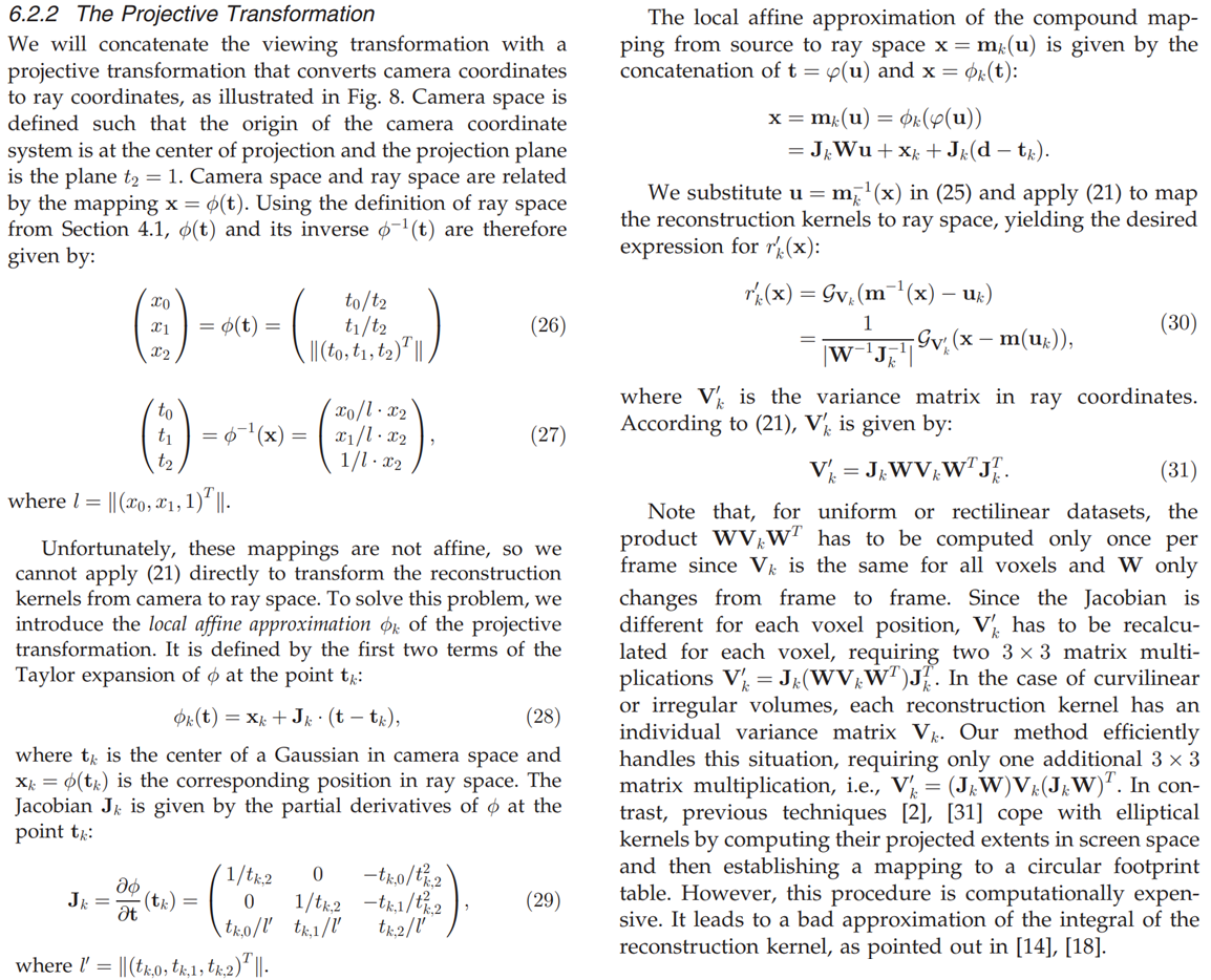
由于近大远小的原理，三维椭球体在二维图片上表现出来不一定是椭圆，而是一种被压扁的形状（下图右下所示）。

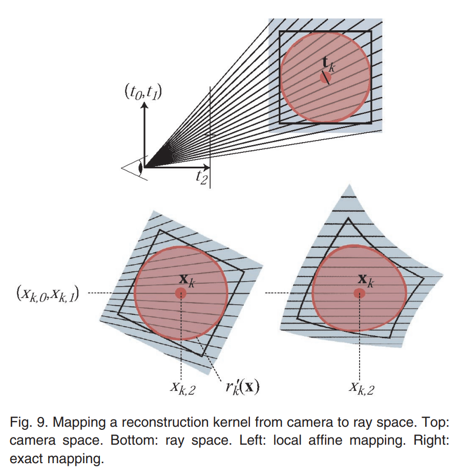
我们想要投影的结果仍然是一个椭圆形。办法是，利用泰勒公式进行近似。论文中$(t_0,t_1,t_2{)}^t$表示相机坐标系下的坐标，$(x_0,x_1)$为像平面坐标系下的二维坐标，$x_2$代表深度（物体到相机中心的距离）。回想一下泰勒公式的标量形式：$$f(x)=f(x_0)+f^{\prime }(x_0)(x-x_0)+\cdots$$将$x\mapsto \mathbf{t}$，$f(x)\mapsto \mathbf{x}$，$x_0\mapsto {\mathbf{t}}_k$，$f(x_0)\mapsto {\mathbf{x}}_k$代入得： x = x k + d x d t ∣ t = t k ( t − t k ) \boldsymbol{x}=\boldsymbol{x}_k+\left.\cfrac{d\boldsymbol{x}}{d\boldsymbol{t}}\right|_{\boldsymbol{t}=\boldsymbol{t}_k}(\boldsymbol{t}-\boldsymbol{t}_k) x=xk​+dtdx​ ​t=tk​​(t−tk​)其中雅可比矩阵 j k = d x d t ∣ t = t k \left.\boldsymbol{j}_k=\cfrac{d\boldsymbol{x}}{d\boldsymbol{t}}\right|_{\boldsymbol{t}=\boldsymbol{t}_k} jk​=dtdx​ ​t=tk​​。注意${\mathbf{x}}_k$和${\mathbf{t}}_k$分别代表二维和三维gaussian中心，必须用原始的精确公式计算。

如果你检查一下论文中出现的${\mathbf{j}}_k$就会发现它是$\mathbf{x}$对$\mathbf{t}$的导。例如，其$(0,0)$项为$\frac{1}{t_{k,2}}$，而$x_0=\frac{t_0}{t_2}$，刚好有$\frac{\partial x_0}{\partial t_2}=\frac{1}{t_2}$，在$\mathbf{t}={\mathbf{t}}_{\mathbf{k}}$时就是$\frac{1}{t_{k,2}}$。

3. computecov3d

根据缩放和旋转计算三维协方差矩阵。比较简单。

// forward method for converting scale and rotation properties of each
// gaussian to a 3d covariance matrix in world space. also takes care
// of quaternion normalization.
__device__ void computecov3d(
	const glm::vec3 scale, // 表示缩放的三维向量
	float mod, // 对应gaussian_renderer/__init__.py中的scaling_modifier
	const glm::vec4 rot, // 表示旋转的四元数
	float* cov3d) // 结果：三维协方差矩阵
{
	// create scaling matrix
	glm::mat3 s = glm::mat3(1.0f);
	s[0][0] = mod * scale.x;
	s[1][1] = mod * scale.y;
	s[2][2] = mod * scale.z;

	// normalize quaternion to get valid rotation
	glm::vec4 q = rot;// / glm::length(rot);
	float r = q.x;
	float x = q.y;
	float y = q.z;
	float z = q.w;

	// compute rotation matrix from quaternion
	glm::mat3 r = glm::mat3(
		1.f - 2.f * (y * y + z * z), 2.f * (x * y - r * z), 2.f * (x * z + r * y),
		2.f * (x * y + r * z), 1.f - 2.f * (x * x + z * z), 2.f * (y * z - r * x),
		2.f * (x * z - r * y), 2.f * (y * z + r * x), 1.f - 2.f * (x * x + y * y)
	);

	glm::mat3 m = s * r;

	// compute 3d world covariance matrix sigma
	glm::mat3 sigma = glm::transpose(m) * m;

	// covariance is symmetric, only store upper right
	cov3d[0] = sigma[0][0];
	cov3d[1] = sigma[0][1];
	cov3d[2] = sigma[0][2];
	cov3d[3] = sigma[1][1];
	cov3d[4] = sigma[1][2];
	cov3d[5] = sigma[2][2];
}

4. preprocesscuda

预处理函数，作用是：

1. 检查gaussian是否可见（在视锥内）；
2. 计算3维、2维协方差矩阵；
3. 把gaussian投影到图像上，计算图像上的中心坐标、半径和覆盖的tile；
4. 计算颜色、深度等杂项。

// perform initial steps for each gaussian prior to rasterization.
template<int c>
__global__ void preprocesscuda(int p, int d, int m,
	const float* orig_points, // 也就是cudarasterizer::rasterizer::forward的means3d
	const glm::vec3* scales,
	const float scale_modifier,
	const glm::vec4* rotations,
	const float* opacities,
	const float* shs,
	bool* clamped,
	const float* cov3d_precomp,
	const float* colors_precomp,
	const float* viewmatrix,
	const float* projmatrix,
	const glm::vec3* cam_pos,
	const int w, int h,
	const float tan_fovx, float tan_fovy,
	const float focal_x, float focal_y,
	int* radii,
	/*上面这些参数的含义都提到过*/
	float2* points_xy_image,  // gaussian中心在图像上的像素坐标
	float* depths, // gaussian中心的深度，即其在相机坐标系的z轴的坐标
	float* cov3ds, // 三维协方差矩阵
	float* rgb, // 根据球谐算出的rgb颜色值
	float4* conic_opacity, // 椭圆对应二次型的矩阵和不透明度的打包存储
	const dim3 grid, // tile的在x、y方向上的数量
	uint32_t* tiles_touched, // gaussian覆盖的tile数量
	bool prefiltered)
{
	auto idx = cg::this_grid().thread_rank(); // 该函数预处理第idx个gaussian
	if (idx >= p)
		return;

	// initialize radius and touched tiles to 0. if this isn't changed,
	// this gaussian will not be processed further.
	radii[idx] = 0;
	tiles_touched[idx] = 0;

	// perform near culling, quit if outside.
	float3 p_view; // gaussian中心在相机坐标系下的坐标
	if (!in_frustum(idx, orig_points, viewmatrix, projmatrix, prefiltered, p_view))
		return; // 不在相机的视锥内就不管了

	// transform point by projecting
	float3 p_orig = { orig_points[3 * idx], orig_points[3 * idx + 1], orig_points[3 * idx + 2] };
	float4 p_hom = transformpoint4x4(p_orig, projmatrix); // homogeneous coordinates（齐次坐标）
	float p_w = 1.0f / (p_hom.w + 0.0000001f); // 想要除以p_hom.w从而转成正常的3d坐标，这里防止除零
	float3 p_proj = { p_hom.x * p_w, p_hom.y * p_w, p_hom.z * p_w };

	// if 3d covariance matrix is precomputed, use it, otherwise compute
	// from scaling and rotation parameters. 
	const float* cov3d;
	if (cov3d_precomp != nullptr)
	{
		cov3d = cov3d_precomp + idx * 6;
	}
	else
	{
		computecov3d(scales[idx], scale_modifier, rotations[idx], cov3ds + idx * 6);
		cov3d = cov3ds + idx * 6;
	}

	// compute 2d screen-space covariance matrix
	float3 cov = computecov2d(p_orig, focal_x, focal_y, tan_fovx, tan_fovy, cov3d, viewmatrix);

	// invert covariance (ewa algorithm)
	float det = (cov.x * cov.z - cov.y * cov.y); // 二维协方差矩阵的行列式
	if (det == 0.0f)
		return;
	float det_inv = 1.f / det; // 行列式的逆
	float3 conic = { cov.z * det_inv, -cov.y * det_inv, cov.x * det_inv };
		// conic是cone的形容词，意为“圆锥的”。猜测这里是指圆锥曲线（椭圆）。
		// 二阶矩阵求逆口诀：“主对调，副相反”。

	// compute extent in screen space (by finding eigenvalues of
	// 2d covariance matrix). use extent to compute a bounding rectangle
	// of screen-space tiles that this gaussian overlaps with. quit if
	// rectangle covers 0 tiles. 
	float mid = 0.5f * (cov.x + cov.z);
	float lambda1 = mid + sqrt(max(0.1f, mid * mid - det));
	float lambda2 = mid - sqrt(max(0.1f, mid * mid - det));
		// 韦达定理求二维协方差矩阵的特征值
	float my_radius = ceil(3.f * sqrt(max(lambda1, lambda2)));
		// 原理见代码后面我的补充说明
		// 这里就是截取gaussian的中心部位（3σ原则），只取像平面上半径为my_radius的部分
	float2 point_image = { ndc2pix(p_proj.x, w), ndc2pix(p_proj.y, h) };
		// ndc2pix(v, s) = ((v + 1) * s - 1) / 2 = (v + 1) / 2 * s - 0.5
	uint2 rect_min, rect_max;
	getrect(point_image, my_radius, rect_min, rect_max, grid);
		// 检查该gaussian在图片上覆盖了哪些tile（由一个tile组成的矩形表示）
	if ((rect_max.x - rect_min.x) * (rect_max.y - rect_min.y) == 0)
		return; // 不与任何tile相交，不管了

	// if colors have been precomputed, use them, otherwise convert
	// spherical harmonics coefficients to rgb color.
	if (colors_precomp == nullptr)
	{
		glm::vec3 result = computecolorfromsh(idx, d, m, (glm::vec3*)orig_points, *cam_pos, shs, clamped);
		rgb[idx * c + 0] = result.x;
		rgb[idx * c + 1] = result.y;
		rgb[idx * c + 2] = result.z;
	}

	// store some useful helper data for the next steps.
	depths[idx] = p_view.z; // 深度，即相机坐标系的z轴
	radii[idx] = my_radius; // gaussian在像平面坐标系下的半径
	points_xy_image[idx] = point_image; // gaussian中心在图像上的像素坐标
	// inverse 2d covariance and opacity neatly pack into one float4
	conic_opacity[idx] = { conic.x, conic.y, conic.z, opacities[idx] };
	tiles_touched[idx] = (rect_max.y - rect_min.y) * (rect_max.x - rect_min.x);
		// gaussian覆盖的tile数量
}

补充说明

❄️(1) 关于二维高斯分布和椭圆的关系，我们可以这么考虑：

二维高斯分布的概率密度函数为$$\begin{array}{c}p(\mathbf{x})=\frac{1}{(2\pi {)}^{\frac{n}{2}}|\sigma {|}^{\frac{1}{2}}}\exp \left\{-\frac{1}{2}(\mathbf{x}-\mathbf{\mu }{)}^t{\sigma }^{-1}(\mathbf{x}-\mathbf{\mu })\right\}\end{array}\text{\hspace{1em}(†)}$$，其中$\mathbf{x}=(x,y{)}^t$，$\sigma$为协方差矩阵，$\mu$为均值。考虑令$p(\mathbf{x})$等于一个常数，并令$\mathbf{u}=\mathbf{x}-\mathbf{\mu }$，即$${\mathbf{u}}^t{\sigma }^{-1}\mathbf{u}=r^2$$其中$r^2$为常数。由于$\sigma$是对称矩阵，一定存在正交矩阵$p$使得$$\sigma =p^t\lambda p$$其中$\lambda =\mathrm{diag}({\lambda }_1,{\lambda }_2)$是由$\sigma$的特征值组成的对角矩阵。带入式$(†)$得$${\mathbf{u}}^t{p}^t{\lambda }^{-1}p\mathbf{u}=r^2$$令$\mathbf{v}=p\mathbf{u}$（也就是相对$\mathbf{u}$坐标系旋转了一个角度），则$${\mathbf{v}}^t{\lambda }^{-1}\mathbf{v}=r^2$$即$$\frac{v_1^2}{{\lambda }_1{r}^2}+\frac{v_2^2}{{\lambda }_2{r}^2}=1$$正好是一个长短轴分别为$\sqrt{{\lambda }_1}r$、$\sqrt{{\lambda }_2}r$的椭圆。令$r=3$就得到了代码中算my_radius的公式。

❄️(2) 关于ndc2pix的解读：

这时候我们必须知道p_proj的真正含义。p_proj是projmatrix乘以gaussian中心的世界坐标p_orig的结果（注意这里所有东西都是转置的，transformpoint4x4(const float3& p, const float* matrix)做的事情实际上是$\left[\begin{array}{cccc}x& y& z& 1\end{array}\right]m$，其中$m$代表matrix（这里是投影矩阵的转置），$x,y,z$代表p）。proj_matrix又是w2c矩阵和投影矩阵的积。我们重点关注投影矩阵。计算投影矩阵的函数为utils/graph_utils.py中的getprojectionmatrix：

def getprojectionmatrix(znear, zfar, fovx, fovy):
    tanhalffovy = math.tan((fovy / 2))
    tanhalffovx = math.tan((fovx / 2))

    top = tanhalffovy * znear
    bottom = -top
    right = tanhalffovx * znear
    left = -right

    p = torch.zeros(4, 4)

    z_sign = 1.0

    p[0, 0] = 2.0 * znear / (right - left)
    p[1, 1] = 2.0 * znear / (top - bottom)
    p[0, 2] = (right + left) / (right - left)
    p[1, 2] = (top + bottom) / (top - bottom)
    p[3, 2] = z_sign
    p[2, 2] = z_sign * zfar / (zfar - znear)
    p[2, 3] = -(zfar * znear) / (zfar - znear)
    return p

这个函数写的极其怪异，p[0,2]和p[1,2]显然为$0$，不知道作者的用意是什么。回想znear和zfar代表该相机能看到的最近和最远距离。注意矩阵$p$是从相机坐标系到像平面二维坐标系的映射，可以表示为 p = [ 1 t a n h a l f f o v x 0 0 0 0 1 t a n h a l f f o v y 0 0 0 0 z f a r z f a r − z n e a r z f a r × z n e a r z f a r − z n e a r 0 0 1 0 ] p=\begin{bmatrix} \frac{1}{\mathrm{tanhalffovx}} &0&0&0\\ 0&\frac{1}{\mathrm{tanhalffovy}}&0&0\\ 0&0&\frac{\mathrm{zfar}}{\mathrm{zfar}-\mathrm{znear}}&\frac{\mathrm{zfar}\times\mathrm{znear}}{\mathrm{zfar}-\mathrm{znear}}\\ 0&0&1&0\\ \end{bmatrix} p= ​tanhalffovx1​000​0tanhalffovy1​00​00zfar−znearzfar​1​00zfar−znearzfar×znear​0​ ​所以， p [ x y z 1 ] = [ x t a n h a l f f o v x y t a n h a l f f o v y z f a r ( z − z n e a r ) z f a r − z n e a r z ] p\begin{bmatrix}x\\y\\z\\1\end{bmatrix}= \begin{bmatrix} \cfrac{x}{\mathrm{tanhalffovx}}\\ \\ \cfrac{y}{\mathrm{tanhalffovy}}\\ \\ \cfrac{\mathrm{zfar}(z-\mathrm{znear})}{\mathrm{zfar}-\mathrm{znear}}\\ \\ z \end{bmatrix} p ​xyz1​ ​= ​tanhalffovxx​tanhalffovyy​zfar−znearzfar(z−znear)​z​ ​显然，作者假设相机坐标系的$z$轴与像平面垂直。$p$矩阵把$z$的范围$[\mathrm{znear},\mathrm{zfar}]$映射到$[0,\mathrm{zfar}]$；$x,y$被映射到了像平面上的坐标，其中图像中心在像平面上的坐标为$(0,0)$，图像边缘在像平面上的$x$、$y$坐标为$\pm 1$。同时，作者在结果的第四个元素保留了被映射前的$z$。

函数ndc2pix的作用就是把像平面上的坐标转化为像素坐标（ndc = normalized device coordinates，详见这篇文章）。我们提到，ndc2pix(v, s)等价于(v + 1) / 2 * s - 0.5。首先把范围$[-1,1]$映射为$[0,2]$，再除以$2$得$[0,1]$，乘$s$（等于图像宽度或高度）就转化为了像素坐标，最后$-0.5$映射到像素中心。

❗️注意：我们有四个坐标系：世界坐标系、相机坐标系、像平面坐标系、图像坐标系，关系如图：

5. render和rendercuda

void forward::render(
	const dim3 grid, dim3 block,
	const uint2* ranges,
	const uint32_t* point_list,
	int w, int h,
	const float2* means2d,
	const float* colors,
	const float4* conic_opacity,
	float* final_t,
	uint32_t* n_contrib,
	const float* bg_color,
	float* out_color)
{
	rendercuda<num_channels> << <grid, block >> > (
		ranges,
		point_list,
		w, h,
		means2d,
		colors,
		conic_opacity,
		final_t,
		n_contrib,
		bg_color,
		out_color);
		// 一个线程负责一个像素，一个block负责一个tile
}

// main rasterization method. collaboratively works on one tile per
// block, each thread treats one pixel. alternates between fetching 
// and rasterizing data.
// "alternates between fetching and rasterizing data":
// 线程在读取数据（把数据从公用显存拉到block自己的显存）和进行计算之间来回切换，
// 使得线程们可以共同读取gaussian数据。
// 这样做的原因是block共享内存比公共显存快得多。
template <uint32_t channels> // channels取3，即rgb三个通道
__global__ void __launch_bounds__(block_x * block_y)
rendercuda(
	const uint2* __restrict__ ranges, // 每个tile对应排过序的数组中的哪一部分
	const uint32_t* __restrict__ point_list, // 按tile、深度排序后的gaussian id列表
	int w, int h, // 图像宽高
	const float2* __restrict__ points_xy_image, // 图像上每个gaussian中心的2d坐标
	const float* __restrict__ features, // rgb颜色
	const float4* __restrict__ conic_opacity, // 解释过了
	float* __restrict__ final_t, // 最终的透光率
	uint32_t* __restrict__ n_contrib,
		// 多少个gaussian对该像素的颜色有贡献（用于反向传播时判断各个gaussian有没有梯度）
	const float* __restrict__ bg_color, // 背景颜色
	float* __restrict__ out_color) // 渲染结果（图片）
{
	// identify current tile and associated min/max pixel range.
	auto block = cg::this_thread_block();
	uint32_t horizontal_blocks = (w + block_x - 1) / block_x; // x方向上tile的个数
	uint2 pix_min = { block.group_index().x * block_x, block.group_index().y * block_y };
		// 我负责的tile的坐标较小的那个角的坐标
	uint2 pix_max = { min(pix_min.x + block_x, w), min(pix_min.y + block_y , h) };
		// 我负责的tile的坐标较大的那个角的坐标
	uint2 pix = { pix_min.x + block.thread_index().x, pix_min.y + block.thread_index().y };
		// 我负责哪个像素
	uint32_t pix_id = w * pix.y + pix.x;
		// 我负责的像素在整张图片中排行老几
	float2 pixf = { (float)pix.x, (float)pix.y }; // pix的浮点数版本

	// check if this thread is associated with a valid pixel or outside.
	bool inside = pix.x < w && pix.y < h; // 看看我负责的像素有没有跑到图像外面去
	// done threads can help with fetching, but don't rasterize
	bool done = !inside;

	// load start/end range of ids to process in bit sorted list.
	uint2 range = ranges[block.group_index().y * horizontal_blocks + block.group_index().x];
	const int rounds = ((range.y - range.x + block_size - 1) / block_size);
		// block_size = 16 * 16 = 256
		// 我要把任务分成rounds批，每批处理block_size个gaussians
		// 每一批，每个线程负责读取一个gaussian的信息，
		// 所以该block的256个线程每一批就可以读取256个gaussian的信息
	int todo = range.y - range.x; // 我要处理的gaussian个数

	// allocate storage for batches of collectively fetched data.
	// __shared__: 同一block中的线程共享的内存
	__shared__ int collected_id[block_size];
	__shared__ float2 collected_xy[block_size];
	__shared__ float4 collected_conic_opacity[block_size];

	// initialize helper variables
	float t = 1.0f; // t = transmittance，透光率
	uint32_t contributor = 0; // 多少个gaussian对该像素的颜色有贡献
	uint32_t last_contributor = 0; // 比contributor慢半拍的变量
	float c[channels] = { 0 }; // 渲染结果

	// iterate over batches until all done or range is complete
	for (int i = 0; i < rounds; i++, todo -= block_size)
	{
		// end if entire block votes that it is done rasterizing
		int num_done = __syncthreads_count(done);
			// 它首先具有__syncthreads的功能（让所有线程回到同一个起跑线上），
			// 并且返回对于多少个线程来说done是true。
		if (num_done == block_size)
			break; // 全干完了，收工

		// collectively fetch per-gaussian data from global to shared
		// 由于当前block的线程要处理同一个tile，所以它们面对的gaussians也是相同的
		// 因此合作读取block_size条的数据。
		// 之所以分批而不是一次读完可能是因为block的共享内存空间有限。
		int progress = i * block_size + block.thread_rank();
		if (range.x + progress < range.y) // 我还有没有活干
		{
			// 读取我负责的gaussian信息
			int coll_id = point_list[range.x + progress];
			collected_id[block.thread_rank()] = coll_id;
			collected_xy[block.thread_rank()] = points_xy_image[coll_id];
			collected_conic_opacity[block.thread_rank()] = conic_opacity[coll_id];
		}
		block.sync(); // 这下collected_*** 数组就被填满了

		// iterate over current batch
		for (int j = 0; !done && j < min(block_size, todo); j++)
		{
			// keep track of current position in range
			contributor++;

			// 下面计算当前gaussian的不透明度
			// resample using conic matrix (cf. "surface 
			// splatting" by zwicker et al., 2001)
			float2 xy = collected_xy[j]; // gaussian中心
			float2 d = { xy.x - pixf.x, xy.y - pixf.y };
				// 该像素到gaussian中心的位移向量
			float4 con_o = collected_conic_opacity[j];
			float power = -0.5f * (con_o.x * d.x * d.x + con_o.z * d.y * d.y) - con_o.y * d.x * d.y;
				// 二维高斯分布公式的指数部分（见补充说明）
			if (power > 0.0f)
				continue;

			// eq. (2) from 3d gaussian splatting paper.
			// obtain alpha by multiplying with gaussian opacity
			// and its exponential falloff from mean.
			// avoid numerical instabilities (see paper appendix). 
			float alpha = min(0.99f, con_o.w * exp(power));
				// gaussian对于这个像素点来说的不透明度
				// 注意con_o.w是”opacity“，是gaussian整体的不透明度
			if (alpha < 1.0f / 255.0f) // 不透明度太小，不渲染
				continue;
			float test_t = t * (1 - alpha); // 透光率是累乘
			if (test_t < 0.0001f)
			{ // 当透光率很低的时候，就不继续渲染了（反正渲染了也看不见）
				done = true;
				continue;
			}

			// eq. (3) from 3d gaussian splatting paper.
			for (int ch = 0; ch < channels; ch++)
				c[ch] += features[collected_id[j] * channels + ch] * alpha * t;
				// 计算当前gaussian对像素颜色的贡献

			t = test_t; // 更新透光率

			// keep track of last range entry to update this
			// pixel.
			last_contributor = contributor;
		}
	}

	// all threads that treat valid pixel write out their final
	// rendering data to the frame and auxiliary buffers.
	if (inside)
	{
		final_t[pix_id] = t;
		n_contrib[pix_id] = last_contributor;
		for (int ch = 0; ch < channels; ch++)
			out_color[ch * h * w + pix_id] = c[ch] + t * bg_color[ch];
			// 把渲染出来的像素值写进out_color
	}
}

补充说明

二维高斯分布的指数部分为$$-\frac{1}{2}{\mathbf{d}}^t{\sigma }^{-1}\mathbf{d}$$其中$\mathbf{d}$就是代码中的d（像素到gaussian中心的位移向量），${\sigma }^{-1}=\left[\begin{array}{cc}con\_o.x& con\_o.y\\ con\_o.y& con\_o.z\end{array}\right]$。把矩阵乘开就得到了代码中的-0.5f * (con_o.x * d.x * d.x + con_o.z * d.y * d.y) - con_o.y * d.x * d.y。

至于为什么不乘前面的常数$\frac{1}{(2\pi {)}^{\frac{n}{2}}|\sigma {|}^{\frac{1}{2}}}$呢？因为con_o.w（即opacity）是可学习的参数，这个常量可以包括进去。

---

下一部分：【计算机视觉】gaussian splatting源码解读补充（三）