1. 理解决策树的基本概念
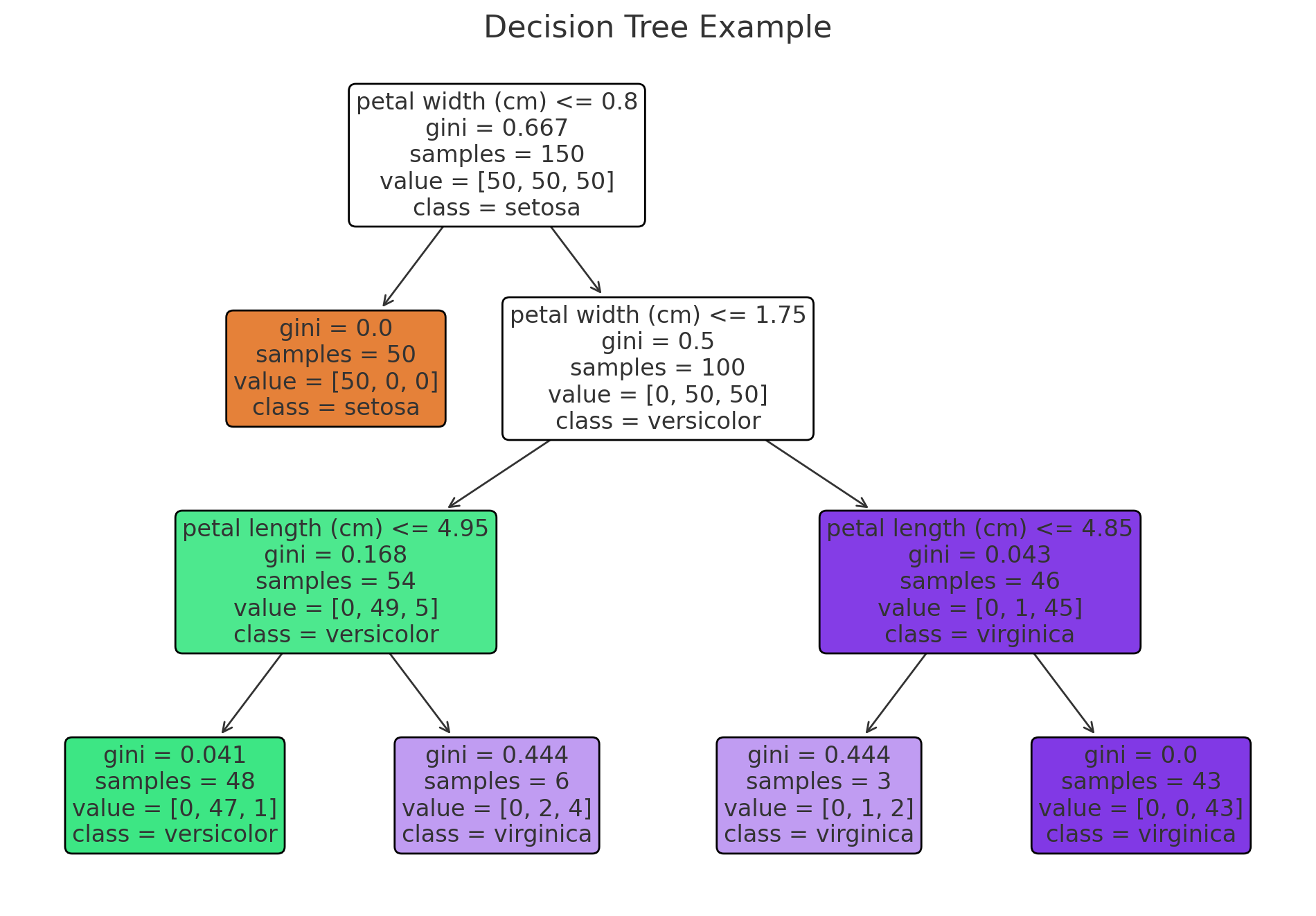
决策树是一种监督学习算法,可以用于分类和回归任务。决策树通过一系列规则将数据划分为不同的类别或值。树的每个节点表示一个特征,节点之间的分支表示特征的可能取值,叶节点表示分类或回归结果。
2. 决策树的构建过程
2.1. 特征选择
特征选择是构建决策树的第一步,通常使用信息增益、基尼指数或增益率等指标。
- 信息增益(information gain)
信息增益表示通过某个特征将数据集划分后的纯度增加量,公式如下:

其中:
d 是数据集。
a 是特征。
v(a) 是特征 a 的所有可能取值。
dv 是数据集中特征 a 取值为 v 的子集。
∣dv∣ 是 dv 中样本的数量。
∣d∣ 是数据集 d 中样本的总数量。
entropy(d) 是数据集 d 的熵,表示数据集本身的纯度。
选择信息增益最大的特征作为当前节点的划分特征。
熵的计算公式为:
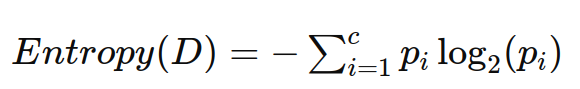
其中:
c 是类别的数量。
pi 是数据集中属于第 i 类的样本所占的比例。
以下代码展示了如何计算熵、信息增益,并选择最优特征。
import numpy as np
from collections import counter
from sklearn.datasets import load_iris

def entropy(y):
    hist = np.bincount(y)
    ps = hist / len(y)
    return -np.sum([p * np.log2(p) for p in ps if p > 0])

def information_gain(x, y, feature):
    # entropy before split
    entropy_before = entropy(y)

    # values and counts
    values, counts = np.unique(x[:, feature], return_counts=true)

    # weighted entropy after split
    entropy_after = 0
    for v, count in zip(values, counts):
        entropy_after += (count / len(y)) * entropy(y[x[:, feature] == v])

    return entropy_before - entropy_after

def best_feature_by_information_gain(x, y):
    features = x.shape[1]
    gains = [information_gain(x, y, feature) for feature in range(features)]
    return np.argmax(gains), max(gains)

# load dataset
iris = load_iris()
x = iris.data
y = iris.target

# find best feature
best_feature, best_gain = best_feature_by_information_gain(x, y)
print(f'best feature: {iris.feature_names[best_feature]}, information gain: {best_gain}')
- 基尼指数(gini index)
也称为基尼不纯度(gini impurity),是一种衡量数据集纯度的指标。基尼指数越小,数据集的纯度越高。
基尼指数的计算公式:
对于一个包含 k 个类别的分类问题,基尼指数 g(d) 定义如下:
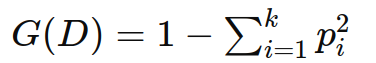
其中:
d 是数据集。
k 是类别的数量。
pi 是数据集中属于第 i 类的样本所占的比例。
条件基尼指数:
在某个特征 a 的条件下,数据集 d 的条件基尼指数 g(d∣a) 定义如下:
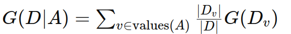
其中:
values(a) 是特征 a 的所有可能取值。
dv 是数据集中特征 a 取值为 v 的子集。
∣dv∣ 是 dv 中样本的数量。
∣d∣ 是数据集 d 中样本的总数量。
g(dv) 是子集 dv 的基尼指数。
基尼增益(gini gain):
基尼增益 gg(d,a) 是通过特征 a 划分数据集 d 后基尼指数的减少量。计算公式如下:
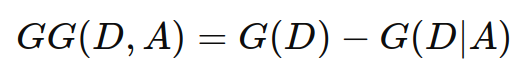
参数解释
d:整个数据集,包含了所有的样本。
a:某个特征,用于划分数据集。
g(d):数据集 d 的基尼指数,表示数据集本身的纯度。
g(d∣a):在特征 a 的条件下,数据集 d 的条件基尼指数,表示在特征 a 的条件下数据集的纯度。
选择基尼增益最大的特征及其分割点作为当前节点的划分特征。
以下代码展示如何使用上述步骤来选择基尼增益最大的特征:
import numpy as np
from sklearn.datasets import load_iris

def gini(y):
    hist = np.bincount(y)
    ps = hist / len(y)
    return 1 - np.sum([p**2 for p in ps if p > 0])

def gini_gain(x, y, feature):
    # gini index before split
    gini_before = gini(y)

    # values and counts
    values, counts = np.unique(x[:, feature], return_counts=true)

    # weighted gini after split
    gini_after = 0
    for v, count in zip(values, counts):
        gini_after += (count / len(y)) * gini(y[x[:, feature] == v])

    return gini_before - gini_after

def best_feature_by_gini_gain(x, y):
    features = x.shape[1]
    gains = [gini_gain(x, y, feature) for feature in range(features)]
    return np.argmax(gains), max(gains)

# load dataset
iris = load_iris()
x = iris.data
y = iris.target

# find best feature
best_feature, best_gain = best_feature_by_gini_gain(x, y)
print(f'best feature: {iris.feature_names[best_feature]}, gini gain: {best_gain}')
- 增益率(gain ratio)
决策树中的增益率(gain ratio)用于选择最优的划分属性,以便构建决策树。增益率是基于信息增益(information gain)的一个修正版本,用于克服信息增益在处理属性取值多样性时可能出现的偏向问题。
信息增益是指选择某一属性划分数据集后,信息熵的减少量。信息增益公式为:
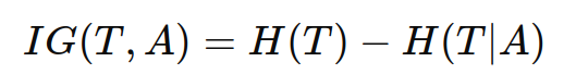
其中:
ig(t,a):属性 a 对数据集 t 的信息增益。
h(t):数据集 t 的熵。
h(t∣a):在给定属性 a 的条件下数据集 t 的条件熵。
增益率通过将信息增益除以属性的固有值(intrinsic value)来计算。固有值是衡量属性取值多样性的一种指标。增益率公式为:
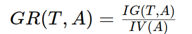
其中:
gr(t,a):属性 a 对数据集 t 的增益率。
ig(t,a):属性 a 对数据集 t 的信息增益。
iv(a):属性 a 的固有值。
固有值(intrinsic value)
固有值反映了属性的取值多样性,计算公式为:
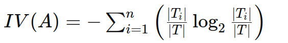
其中:
ti:属性 a 的第 i 个取值所对应的样本子集。
∣ti∣:属性 a 的第 i 个取值所对应的样本子集的样本数量。
∣t∣:数据集 t 的总样本数量。
n:属性 a 取值的个数。
通过计算每个属性的增益率,选择增益率最高的属性作为决策树节点的划分属性,从而构建最优的决策树。
2.2. 划分节点
根据选定的特征和阈值,数据集被划分成多个子集。
2.3. 递归构建
递归地对每个子集进行特征选择和划分,直到满足停止条件(如当前数据子集中的所有实例都属于同一个类别,或达到预设的最大树深度)。
特征选择以增益率为例,在决策树构建过程中,选择每个节点的分裂特征是基于当前数据集的增益率计算结果的。对于每个分裂点,我们都会重新计算剩余特征的增益率,并选择其中最高的作为下一个分裂特征。
import numpy as np
import pandas as pd

# 计算熵
def entropy(y):
    unique_labels, counts = np.unique(y, return_counts=true)
    probabilities = counts / counts.sum()
    return -np.sum(probabilities * np.log2(probabilities))

# 计算信息增益
def information_gain(data, split_attribute, target_attribute):
    total_entropy = entropy(data[target_attribute])
    values, counts = np.unique(data[split_attribute], return_counts=true)
    weighted_entropy = np.sum([
        (counts[i] / np.sum(counts)) * entropy(data[data[split_attribute] == values[i]][target_attribute])
        for i in range(len(values))
    ])
    info_gain = total_entropy - weighted_entropy
    return info_gain

# 计算固有值
def intrinsic_value(data, split_attribute):
    values, counts = np.unique(data[split_attribute], return_counts=true)
    probabilities = counts / counts.sum()
    return -np.sum(probabilities * np.log2(probabilities))

# 计算增益率
def gain_ratio(data, split_attribute, target_attribute):
    info_gain = information_gain(data, split_attribute, target_attribute)
    iv = intrinsic_value(data, split_attribute)
    return info_gain / iv if iv != 0 else 0

# 递归构建决策树
def build_decision_tree(data, original_data, features, target_attribute, parent_node_class=none):
    # 条件1: 所有数据点属于同一类别
    if len(np.unique(data[target_attribute])) <= 1:
        return np.unique(data[target_attribute])[0]

    # 条件2: 数据子集为空
    elif len(data) == 0:
        return np.unique(original_data[target_attribute])[np.argmax(np.unique(original_data[target_attribute], return_counts=true)[1])]

    # 条件3: 没有更多的特征可以分裂
    elif len(features) == 0:
        return parent_node_class

    else:
        parent_node_class = np.unique(data[target_attribute])[np.argmax(np.unique(data[target_attribute], return_counts=true)[1])]

        gain_ratios = {feature: gain_ratio(data, feature, target_attribute) for feature in features}
        best_feature = max(gain_ratios, key=gain_ratios.get)

        tree = {best_feature: {}}

        features = [i for i in features if i != best_feature]

        for value in np.unique(data[best_feature]):
            sub_data = data[data[best_feature] == value]
            subtree = build_decision_tree(sub_data, original_data, features, target_attribute, parent_node_class)
            tree[best_feature][value] = subtree

        return tree

# 可视化决策树
def visualize_tree(tree, depth=0):
    if isinstance(tree, dict):
        for attribute, subtree in tree.items():
            if isinstance(subtree, dict):
                for value, subsubtree in subtree.items():
                    print(f"{'|   ' * depth}|--- {attribute} = {value}")
                    visualize_tree(subsubtree, depth + 1)
            else:
                print(f"{'|   ' * depth}|--- {attribute} = {value}: {subtree}")
    else:
        print(f"{'|   ' * depth}|--- {tree}")

# 示例数据
data = pd.dataframe({
    'outlook': ['sunny', 'sunny', 'overcast', 'rain', 'rain', 'rain', 'overcast', 'sunny', 'sunny', 'rain', 'sunny', 'overcast', 'overcast', 'rain'],
    'temperature': ['hot', 'hot', 'hot', 'mild', 'cool', 'cool', 'cool', 'mild', 'cool', 'mild', 'mild', 'mild', 'hot', 'mild'],
    'humidity': ['high', 'high', 'high', 'high', 'normal', 'normal', 'normal', 'high', 'normal', 'normal', 'normal', 'high', 'normal', 'high'],
    'wind': ['weak', 'strong', 'weak', 'weak', 'weak', 'strong', 'strong', 'weak', 'weak', 'weak', 'strong', 'strong', 'weak', 'strong'],
    'playtennis': ['no', 'no', 'yes', 'yes', 'yes', 'no', 'yes', 'no', 'yes', 'yes', 'yes', 'yes', 'yes', 'no']
})

# 构建决策树
features = ['outlook', 'temperature', 'humidity', 'wind']
target_attribute = 'playtennis'
tree = build_decision_tree(data, data, features, target_attribute)

# 可视化决策树
print("decision tree:")
visualize_tree(tree)
通过运行代码,可以看到每个节点选择的分裂特征以及决策树的结构:
decision tree:
|--- temperature = cool
|   |--- playtennis = yes
|--- temperature = hot
|   |--- playtennis = no
|--- temperature = mild
|   |--- outlook = sunny
|   |   |--- humidity = high
|   |   |   |--- playtennis = no
|   |   |--- humidity = normal
|   |   |   |--- playtennis = yes
|   |--- outlook = rain
|   |   |--- wind = weak
|   |   |   |--- playtennis = yes
|   |   |--- wind = strong
|   |   |   |--- playtennis = no
|   |--- outlook = overcast
|   |   |--- playtennis = yes
解释决策树的结构:
根节点是 temperature,这是第一个选择的分裂特征。
temperature 的每个取值(cool, hot, mild)对应一个子节点。
如果 temperature 是 cool,则 playtennis 是 yes。
如果 temperature 是 hot,则 playtennis 是 no。
如果 temperature 是 mild,则继续分裂 outlook 属性:
    outlook 是 sunny 时,进一步分裂 humidity 属性:
        humidity 是 high 时,playtennis 是 no。
        humidity 是 normal 时,playtennis 是 yes。
    outlook 是 rain 时,进一步分裂 wind 属性:
        wind 是 weak 时,playtennis 是 yes。
        wind 是 strong 时,playtennis 是 no。
    outlook 是 overcast 时,playtennis 是 yes。
通过这种方式,决策树会根据每个节点选择最佳的分裂特征,直到所有数据点都被正确分类或没有更多的特征可供分裂。
2.4. 防止过拟合
防止决策树过拟合的方法主要包括剪枝、设置深度限制和样本数量限制。以下是一些常用的方法及其实现:
- 预剪枝 (pre-pruning)
预剪枝是在构建决策树时限制树的增长。常用的方法包括:
设置最大深度:限制树的深度,防止树过深导致过拟合。
设置最小样本分裂数:如果节点中的样本数小于某个阈值,则不再分裂该节点。
设置最小信息增益:如果信息增益小于某个阈值,则不再分裂该节点。
- 后剪枝 (post-pruning)
后剪枝是在决策树完全生长后,剪去一些不重要的分支。常用的方法包括:
代价复杂度剪枝 (cost complexity pruning):基于一个代价复杂度参数 α,剪去那些对降低训练误差贡献较小但增加了模型复杂度的分支。
代价复杂度剪枝 (ccp) 是一种后剪枝技术,用于简化已经完全生长的决策树。ccp 通过引入一个复杂度惩罚参数 α 来权衡决策树的复杂度与其在训练集上的误差。通过调整 α,我们可以控制模型的复杂度,防止过拟合。
原理
ccp 的基本思想是通过最小化以下代价复杂度函数来选择最佳的子树:
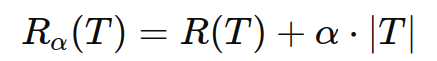
其中:
rα(t) 是带有复杂度惩罚项的代价复杂度。
r(t)是子树 t 的误差。
α 是复杂度惩罚项,控制模型复杂度与误差之间的权衡。
∣t∣ 是子树 t 的叶节点数量。
较小的 α 值允许更多的节点,使树更加复杂;较大的 α 值会剪去更多的节点,使树更加简单。
代价复杂度剪枝步骤:
构建完全生长的决策树:首先,生成一棵完全生长的决策树,使其充分拟合训练数据。
计算每个子树的误差:对子树中的所有节点计算其误差 r(t)。
计算代价复杂度:对于每个子树,计算其代价复杂度 rα(t)。
选择合适的 α:通过关系图或交叉验证结果选择最佳的 α 值。
剪枝:根据选定的 α 值,剪去那些对降低误差贡献不大但增加了复杂度的节点。
import numpy as np
import pandas as pd
from sklearn.tree import decisiontreeclassifier, export_text
import matplotlib.pyplot as plt

# 示例数据
data = pd.dataframe({
    'outlook': ['sunny', 'sunny', 'overcast', 'rain', 'rain', 'rain', 'overcast', 'sunny', 'sunny', 'rain', 'sunny', 'overcast', 'overcast', 'rain'],
    'temperature': ['hot', 'hot', 'hot', 'mild', 'cool', 'cool', 'cool', 'mild', 'cool', 'mild', 'mild', 'mild', 'hot', 'mild'],
    'humidity': ['high', 'high', 'high', 'high', 'normal', 'normal', 'normal', 'high', 'normal', 'normal', 'normal', 'high', 'normal', 'high'],
    'wind': ['weak', 'strong', 'weak', 'weak', 'weak', 'strong', 'strong', 'weak', 'weak', 'weak', 'strong', 'strong', 'weak', 'strong'],
    'playtennis': ['no', 'no', 'yes', 'yes', 'yes', 'no', 'yes', 'no', 'yes', 'yes', 'yes', 'yes', 'yes', 'no']
})

# 将特征和目标变量转换为数值编码
data_encoded = pd.get_dummies(data[['outlook', 'temperature', 'humidity', 'wind']])
target = data['playtennis'].apply(lambda x: 1 if x == 'yes' else 0)

# 拆分数据集
x = data_encoded
y = target

# 构建完全生长的决策树
clf = decisiontreeclassifier(random_state=0)
clf.fit(x, y)

# 导出决策树规则
tree_rules = export_text(clf, feature_names=list(data_encoded.columns))
print("original decision tree rules:")
print(tree_rules)

# 计算代价复杂度剪枝路径
path = clf.cost_complexity_pruning_path(x, y)
ccp_alphas, impurities = path.ccp_alphas, path.impurities

# 训练不同复杂度惩罚项的决策树
clfs = []
for ccp_alpha in ccp_alphas:
    clf = decisiontreeclassifier(random_state=0, ccp_alpha=ccp_alpha)
    clf.fit(x, y)
    clfs.append(clf)

# 绘制复杂度惩罚项与树结构的关系图
node_counts = [clf.tree_.node_count for clf in clfs]
depth = [clf.tree_.max_depth for clf in clfs]

fig, ax = plt.subplots(3, 1, figsize=(10, 10))
ax[0].plot(ccp_alphas, node_counts, marker='o', drawstyle="steps-post")
ax[0].set_xlabel("alpha")
ax[0].set_ylabel("number of nodes")
ax[0].set_title("number of nodes vs alpha")

ax[1].plot(ccp_alphas, depth, marker='o', drawstyle="steps-post")
ax[1].set_xlabel("alpha")
ax[1].set_ylabel("depth")
ax[1].set_title("depth vs alpha")

ax[2].plot(ccp_alphas, impurities, marker='o', drawstyle="steps-post")
ax[2].set_xlabel("alpha")
ax[2].set_ylabel("impurity")
ax[2].set_title("impurity vs alpha")

plt.tight_layout()
plt.show()

# 选择合适的 alpha 进行剪枝并可视化决策树,例如选择 impurity 最小对应的 alpha
# impurity 反映了决策树在分裂节点时的纯度,纯度越高(impurity 越低),节点中样本越一致,分类效果越好。
optimal_alpha = ccp_alphas[np.argmin(impurities)]
pruned_tree = decisiontreeclassifier(random_state=0, ccp_alpha=optimal_alpha)
pruned_tree.fit(x, y)

# 导出剪枝后的决策树规则
pruned_tree_rules = export_text(pruned_tree, feature_names=list(data_encoded.columns))

print("pruned decision tree rules:")
print(pruned_tree_rules)
3. 使用集成方法
- 随机森林:通过构建多棵决策树并结合它们的预测结果,可以减少单棵树的过拟合。
使用随机森林(random forest)是一种有效的方法来防止单个决策树模型的过拟合问题。随机森林通过构建多棵决策树并集成它们的预测结果,从而提高模型的泛化能力。
随机森林防止过拟合的机制:
1. 集成学习:
    随机森林是一种集成学习方法,通过构建多棵决策树,并将它们的预测结果进行投票或平均,从而得到最终的预测结果。这种方式可以有效地减少单棵决策树的高方差,提高模型的稳定性和泛化能力。

2. 随机特征选择:
    在每棵决策树的节点分裂时,随机森林不会考虑所有特征,而是从所有特征中随机选择一个子集来进行分裂。这样可以减少树之间的相关性,提高集成效果。

3. bootstrap 重采样:
    每棵决策树都是通过对原始训练数据进行 bootstrap 重采样(有放回抽样)得到的不同样本集进行训练。这样每棵树都有不同的训练数据,进一步减少了树之间的相关性。
- 梯度提升树:通过逐步构建一系列决策树,每棵树修正前一棵树的错误,可以提高模型的泛化能力。
梯度提升树(gradient boosting trees, gbt)是一种集成学习方法,通过逐步构建一系列决策树来提高模型的预测性能。每棵新树的构建是为了修正之前所有树的误差。
梯度提升树防止过拟合的机制:
1. 分阶段训练:
    梯度提升树采用逐步训练的方法。每次构建新树时,模型会根据之前所有树的预测误差来调整新树的结构。这种逐步优化的方法可以有效减少过拟合。

2. 学习率:
    学习率(learning rate)控制每棵树对最终模型的贡献。较小的学习率使得每棵树的影响较小,从而需要更多的树来拟合训练数据。尽管这会增加计算成本,但可以显著降低过拟合的风险。

3. 树的深度:
    限制每棵树的最大深度可以防止单棵树过于复杂,从而避免过拟合。浅层树(通常 3-5 层)虽然不能完全拟合数据,但可以捕捉到数据的主要结构,从而与其他树一起构成一个强大的集成模型。

4. 子样本采样:
    在构建每棵树时,梯度提升树可以对训练数据进行子样本采样(subsampling)。这种方法通过引入训练数据的随机性,减少了模型的方差,从而防止过拟合。

5. 正则化:
    梯度提升树可以引入正则化参数,如 l1 和 l2 正则化,来进一步防止模型的过拟合。
4. 实际应用中的决策树
决策树可以用于多个实际应用,如客户分类、疾病诊断、风险评估等。在实际应用中,需要根据具体问题调整决策树的参数(如树的最大深度、最小样本分裂数等),以达到最佳效果。
发表评论