David Silver Lecture 3: planning by dynamic programming

1 introduction

1.1 定义

定义：

核心思想：
将复杂问题拆解成简单子问题

1.2 requirements for dynamic programming

• optimal substructure
  • principle of optimality applies
  • optimal solution can be decomposed into subproblems
• overlapping subproblems
  • subproblem会调用很多次
  • solution需要存储起来和进行复用
• mdp 满足以下性质
  • bellman 方程提供递归的分解
  • value 函数存储和复用solutions

1.3 planning by dynamic programming

几种假设：
1）dp 假设对mdp可观测结果
2）for prediction

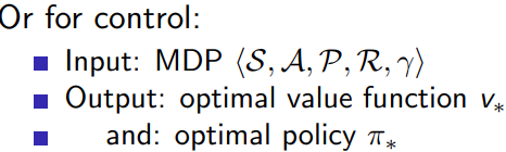
3)for control

1.4 动态规划的其他应用

• scheduling algorithm
• string algorithms (e.g. sequence alignment)
• graph algorithms (e.g. shortest path algorithms)
• graphical models (e.g. viterbi algorithm)
• bioinformatics (e.g. lattice models)

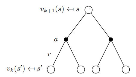
2 policy evaluation

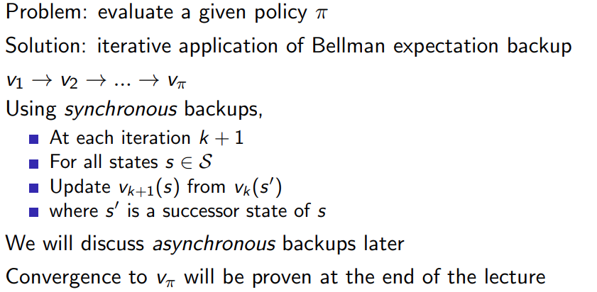
动态问题的结构可以拆成下面三个部分：
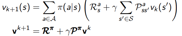
state transition s n = f ( s n − 1 , a n ) value function j ∗ ( s ) = min ⁡ a ∈ a { l ( s , a ) + γ ∑ s ′ ∈ s p ( s ′ ∣ s , a ) j ∗ ( s ′ ) } policy π ( s ) = arg ⁡ min ⁡ a { l ( s , a ) + γ ∑ s ′ ∈ s p ( s ′ ∣ s , a ) j ∗ ( s ′ ) } \begin{aligned} \text{state transition} & \quad s_{n} = f(s_{n-1}, a_{n}) \\ \text{value function} & \quad j^*(s) = \min \limits_{a\in a} \{l(s,a)+\gamma \sum_{s' \in s} p(s' | s, a) j^*(s')\} \\ \text{policy} & \quad \pi(s)=\arg\min \limits_{a} \{l(s,a)+\gamma \sum_{s' \in s} p(s' | s, a) j^*(s')\} \end{aligned} state transitionvalue functionpolicy​sn​=f(sn−1​,an​)j∗(s)=a∈amin​{l(s,a)+γs′∈s∑​p(s′∣s,a)j∗(s′)}π(s)=argamin​{l(s,a)+γs′∈s∑​p(s′∣s,a)j∗(s′)}​
代码的结构大概是这样的

```matlab
for state = 1:num_state
	for action = 1:nun_action
		q = instaneous_cost(state, action);
		next_state = transition(state, action);
		q = q + j(next_state);
	end
end

用iterative policy evaluation 表示：

% initialize the grid world and parameters
grid_size = 4;
num_actions = 4;
discount_factor = 1.0;
theta = 1e-4;

% initialize state-value function
v = zeros(grid_size);

% define the reward function
reward = -1;

% define the transition probabilities for the uniform random policy
policy = ones(grid_size, grid_size, num_actions) / num_actions;

% iterative policy evaluation
while true
    delta = 0;
    
    % loop over all states
    for i = 1:grid_size
        for j = 1:grid_size
            
            % skip the start and terminal states
            if (i == 1 && j == 1) || (i == grid_size && j == grid_size)
                continue;
            end
            
            % store the old value
            old_value = v(i, j);
            
            % calculate the new value by averaging over actions
            new_value = 0;
            for action = 1:num_actions
                [next_i, next_j] = apply_action(i, j, action);
                reward_next = (next_i == grid_size && next_j == grid_size) * (1 - discount_factor);
                new_value = new_value + policy(i, j, action) * (reward + reward_next + discount_factor * v(next_i, next_j));
            end
            
            % update the value function
            v(i, j) = new_value;
            delta = max(delta, abs(old_value - new_value));
        end
    end
    
    % check for convergence
    if delta < theta
        break;
    end
end

% apply the given action to the current state (i, j)
function [next_i, next_j] = apply_action(i, j, action)
    grid_size = 4;
    
    % actions: 1 = up, 2 = down, 3 = left, 4 = right
    if action == 1
        next_i = max(i - 1, 1);
        next_j = j;
    elseif action == 2
        next_i = min(i + 1, grid_size);
        next_j = j;
    elseif action == 3
        next_i = i;
        next_j = max(j - 1, 1);
    else
        next_i = i;
        next_j = min(j + 1, grid_size);
    end
end

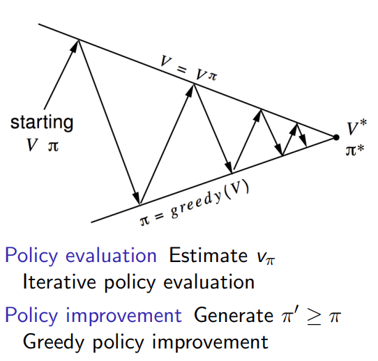
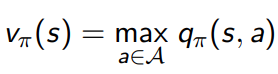
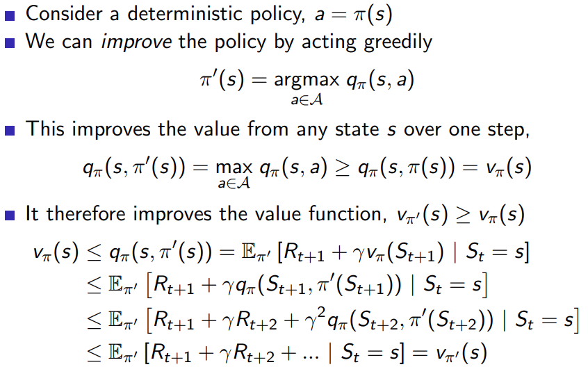
3 policy iteration

3.1 how to improve policy

每一步都找出optimal的value function, 作为state的value function

import numpy as np

def gridworld_policy_iteration():
    n_states = 16
    n_actions = 4
    terminal_state = 15
    rewards = -1 * np.ones((n_states, n_actions))
    rewards[terminal_state, :] = 0

    transition_matrix = np.zeros((n_states, n_actions, n_states))

    for state in range(n_states):
        for action in range(n_actions):
            if state == terminal_state:
                transition_matrix[state, action, state] = 1
                continue

            next_state = state

            if action == 0:  # up
                next_state = max(state - 4, 0)
            elif action == 1:  # down
                next_state = min(state + 4, n_states - 1)
            elif action == 2:  # left
                next_state = state - 1
                if state % 4 == 0:
                    next_state = state
            elif action == 3:  # right
                next_state = state + 1
                if (state + 1) % 4 == 0:
                    next_state = state

            transition_matrix[state, action, next_state] = 1

    gamma = 0.99
    max_iter = 1000
    theta = 1e-10

    policy = np.ones((n_states, n_actions)) / n_actions

    for _ in range(max_iter):
        policy_stable = true

        # policy evaluation
        v = np.zeros(n_states)
        while true:
            delta = 0
            for state in range(n_states):
                v = v[state]
                v[state] = np.sum(policy[state, :] * (rewards[state, :] + gamma * transition_matrix[state, :, :] @ v))
                delta = max(delta, abs(v - v[state]))
            if delta < theta:
                break

        # policy improvement
        for state in range(n_states):
            old_action = np.argmax(policy[state, :])
            action_returns = np.zeros(n_actions)
            for action in range(n_actions):
                action_returns[action] = rewards[state, action] + gamma * np.dot(transition_matrix[state, action, :], v)
            best_action = np.argmax(action_returns)
            policy[state, :] = 0
            policy[state, best_action] = 1

            if old_action != best_action:
                policy_stable = false

        if policy_stable:
            break

    optimal_policy = policy
    state_values = v

    return optimal_policy, state_values

optimal_policy, state_values = gridworld_policy_iteration()
print("optimal policy:")
print(optimal_policy)
print("state values:")
print(state_values)

代码的关键在于

# 找到最大reward对应的action，对其policy为1，其他为0
            for action in range(n_actions):
                action_returns[action] = rewards[state, action] + gamma * np.dot(transition_matrix[state, action, :], v)
            best_action = np.argmax(action_returns)
            policy[state, :] = 0
            policy[state, best_action] = 1

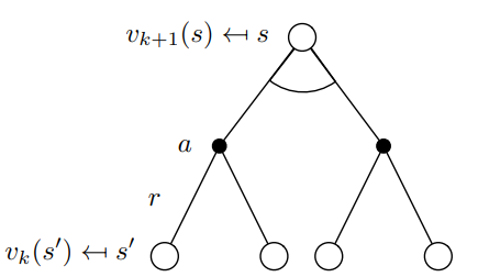
4 value iteration

4.1 value iteration in mdps

4.1.1 principle of optimality

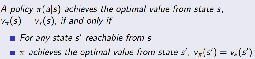
任何的优化策略可以划分成两个组成部分，
1.第一步采用最优动作$a_{\ast }$
2.对successor state采用optimal policy

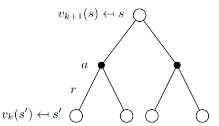
4.1.2 deterministic value iteration

• 子问题的solution $v_{\ast }(s^{\prime })$
• 问题的solution $v_{\ast }(s)$可以通过往前走一步得到
  
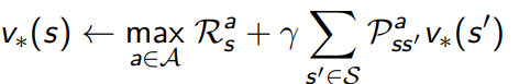
• 直觉理解，start with final rewards and work backwards
• still works with loopy, stochastic mdps
  
  
  
  值迭代的思想非常简单，代码看起来更美观一点

import numpy as np

# gridworld environment
rows = 4
cols = 4
terminal_states = [(0, 0), (rows-1, cols-1)]
actions = [(0, 1), (1, 0), (0, -1), (-1, 0)]

def is_valid_state(state):
    r, c = state
    return 0 <= r < rows and 0 <= c < cols and state not in terminal_states

def next_state(state, action):
    r, c = np.array(state) + np.array(action)
    if is_valid_state((r, c)):
        return r, c
    return state

# value iteration
def value_iteration(gamma=1, theta=1e-6):
    v = np.zeros((rows, cols))
    while true:
        delta = 0
        for r in range(rows):
            for c in range(cols):
                state = (r, c)
                if state in terminal_states:
                    continue

                v = v[state]
                max_value = float('-inf')
                for a in actions:
                    next_s = next_state(state, a)
                    value = -1 + gamma * v[next_s]
                    max_value = max(max_value, value)
                v[state] = max_value
                delta = max(delta, abs(v - v[state]))

        if delta < theta:
            break
    return v

# find optimal policy
def find_optimal_policy(v, gamma=1):
    policy = np.zeros((rows, cols, len(actions)))
    for r in range(rows):
        for c in range(cols):
            state = (r, c)
            if state in terminal_states:
                continue

            q_values = np.zeros(len(actions))
            for i, a in enumerate(actions):
                next_s = next_state(state, a)
                q_values[i] = -1 + gamma * v[next_s]
            optimal_action = np.argmax(q_values)
            policy[state][optimal_action] = 1
    return policy

# find the shortest path using the optimal policy
def find_shortest_path(policy):
    state = (0, 0)
    path = [state]
    while state != (rows-1, cols-1):
        action_idx = np.argmax(policy[state])
        state = next_state(state, actions[action_idx])
        path.append(state)
    return path

v = value_iteration()
policy = find_optimal_policy(v)
path = find_shortest_path(policy)

print("shortest path:", path)

5 extensions to dp

5.1 asynchronous dynamic programming

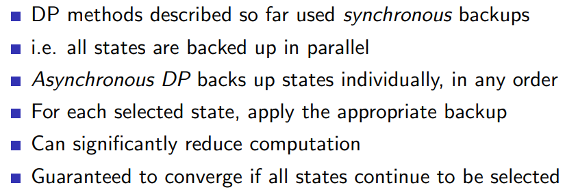
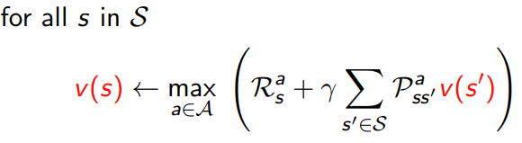
5.1.1 in place dynamic programming

• synchronuous value iteration
  
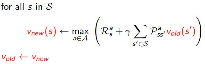
• in place value iteration
  

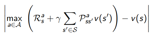
5.1.2 prioritised sweeping

• use magnitude of bellman error to guide state selection, e.g.
  

5.1.3 real time dp

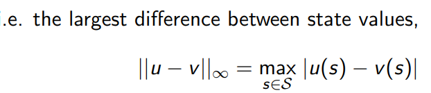
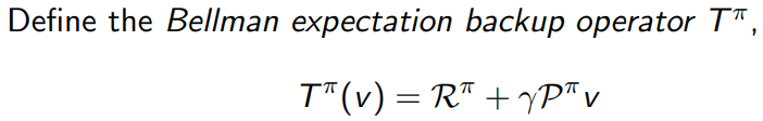
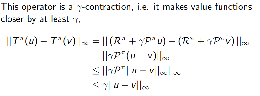
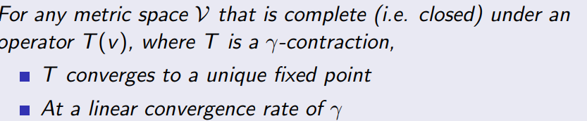
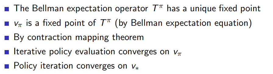
6 contraction mapping

类似于李雅普诺夫稳定性的定义

6.1技术问题

6.2 value function space

6.3 bellman expectation backup is a contraction

总结

• policy evaluation
  $$v(s)=\sum _a\pi (a|s)(r(s,a)+\gamma \sum _{s^{\prime }}p(s^{\prime }|s,a)v(s^{\prime }))$$
  

• policy improvement
  
  找到stable的policy之后停止

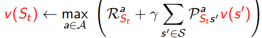
• value iteration
  $$\begin{array}{rl}{v}_{k+1}(s)& =\underset{a}{\max }(r(s,a)+\gamma \sum _{s^{\prime }}p(s^{\prime }|s,a)v_k(s^{\prime }))\\ v_{k+1}(s)& =\underset{a}{\max }r(s,a)+\gamma \sum _{s^{\prime }}p(s^{\prime }|s,a)v_k(s^{\prime })\end{array}$$

• intuition
  将问题拆分成子问题，在使用greedy 策略；

• 李雅普诺夫稳定
  线性收敛，有稳定点，系统最终会收敛到稳定点。