【目标检测】YOLOv5算法实现(六)：评价指标及实现

文章地址：
yolov5算法实现(一)：算法框架概述
yolov5算法实现(二)：模型搭建
yolov5算法实现(三)：数据集加载
yolov5算法实现(四)：正样本匹配与损失计算
yolov5算法实现(五)：预测结果后处理
yolov5算法实现(六)：评价指标及实现
yolov5算法实现(七)：模型训练
yolov5算法实现(八)：模型验证
yolov5算法实现(九)：模型预测

0 引言

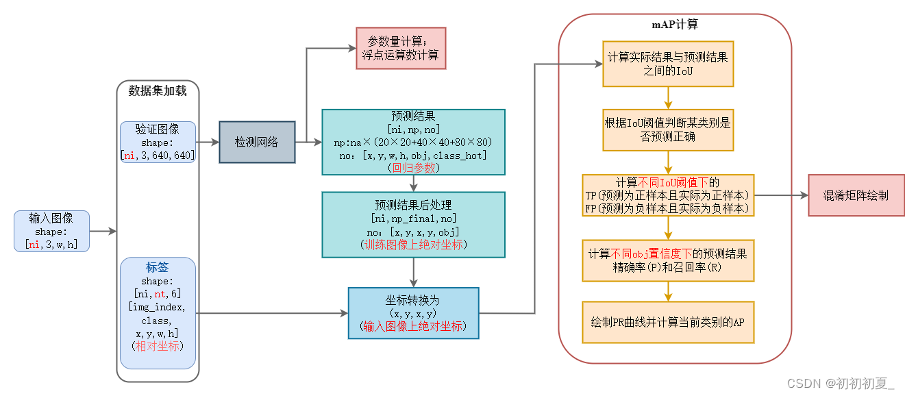
  本篇文章实现目标检测评价指标的实现，主要包含以下几个指标：
   空间复杂度：参数量( parameters )
   时间复杂度：浮点运算数( flops )
   精度：精确率( p )、召回率( r )、混淆矩阵; 均值平均精度( map )

$$p=\frac{tp}{tp+fp}$$
$$r=\frac{tp}{tp+fn}$$
$$\mathrm{m}ap=\frac{\sum ap}{n}$$
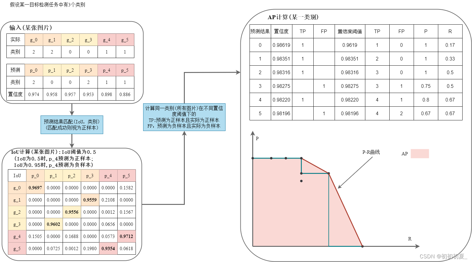
$tp$表示预测为正样本且实际为正样本数量，$fp$表示预测为正样本但实际为负样本数量。在目标检测中，根据iou阈值和类别对预测结果进行和实际标签的匹配，若匹配成功则该检测结果视为$tp$，反之则视为$fp$。$ap$为在不同的类别置信度下，类别$p-r$值围成的曲线面积，$map$为所有类别的$ap$值的平均值。
  假设某目标检测任务中类别数为3，具体的$map$计算过程如图2所示。

1 参数量和浮点运算数计算

def param_flops_cal(model, verbose=false, imgsz=640):
    '''
    打印模型信息
    :param model: 模型
    :param imgsz:
    '''

    n_p = sum(x.numel() for x in model.parameters())  # 参数量
    n_g = sum(x.numel() for x in model.parameters() if x.requires_grad)  # 更新参数量
    
    print(
            f"{'layer':>5} {'name':>40} {'gradient':>9} {'parameters':>12} {'shape':>20} {'mu':>10} {'sigma':>10}")
    for i, (name, p) in enumerate(model.named_parameters()):
        name = name.replace('module_list.', '')
        print('%5g %40s %9s %12g %20s %10.3g %10.3g' %
                  (i, name, p.requires_grad, p.numel(), list(p.shape), p.mean(), p.std()))

    try:  # flops
        p = next(model.parameters())
        stride = max(int(model.stride.max()), 32) if hasattr(model, 'stride') else 32  # max stride
        im = torch.empty((1, p.shape[1], stride, stride), device=p.device)  # input image in bchw format
        flops = thop.profile(deepcopy(model), inputs=(im,), verbose=false)[0] / 1e9 * 2  # stride gflops

        imgsz = imgsz if isinstance(imgsz, list) else [imgsz, imgsz]  # expand if int/float
        fs = f', {flops * imgsz[0] / stride * imgsz[1] / stride:.1f} gflops'  # 640x640 gflops
    except exception:
         fs = ''


    name = path(model.yaml_file).stem.replace('yolov5', 'yolov5') if hasattr(model, 'yaml_file') else 'model'
    printf(f"{name} summary: {len(list(model.modules()))} layers, {n_p}({n_p / 1e6:.2f}m) parameters, {n_g} gradients{fs}")

2 map计算

def ap_per_class(tp, conf, pred_cls, target_cls, plot=false, save_dir='.', names=(), eps=1e-16, prefix=''):
    """ compute the average precision, given the recall and precision curves.
    source: https://github.com/rafaelpadilla/object-detection-metrics.
    # arguments
        tp:  所有预测结果在不同iou下的预测结果 [n, 10]
        conf:  所有预测结果的置信度
        pred_cls:  所有预测结果得到的类别
        target_cls:  所有图片上的实际类别
        plot:  plot precision-recall curve at map@0.5
        save_dir:  plot save directory
    # returns
        the average precision as computed in py-faster-rcnn.
    """

    # sort by objectness
    i = np.argsort(-conf)  # 根据置信度从大到小排序
    tp, conf, pred_cls = tp[i], conf[i], pred_cls[i]

    # 得到所有类别及其对应数量
    unique_classes, nt = np.unique(target_cls, return_counts=true)
    nc = unique_classes.shape[0]  # number of classes

    # create precision-recall curve and compute ap for each class (针对每一个类别计算p,r曲线)
    px, py = np.linspace(0, 1, 1000), []  # for plotting
    ap, p, r = np.zeros((nc, tp.shape[1])), np.zeros((nc, 1000)), np.zeros((nc, 1000))
    for ci, c in enumerate(unique_classes):  # 对每一个类别进行p,r计算
        i = pred_cls == c
        n_l = nt[ci]  # number of labels 该类别的实际数量(正样本数量)
        n_p = i.sum()  # number of predictions 预测结果数量
        if n_p == 0 or n_l == 0:
            continue

        # accumulate fps and tps, cumsum 轴向的累加和
        fpc = (1 - tp[i]).cumsum(0)  # fp累加和(预测为负样本且实际为负样本)
        tpc = tp[i].cumsum(0)  # tp累加和(预测为正样本且实际为正样本)

        # recall
        recall = tpc / (n_l + eps)  # recall curve
        r[ci] = np.interp(-px, -conf[i], recall[:, 0], left=0)  # 在不同置信度下的召回率

        # precision
        precision = tpc / (tpc + fpc)  # precision curve
        p[ci] = np.interp(-px, -conf[i], precision[:, 0], left=1)  # 在不同置信度下的精确率

        # ap from recall-precision curve(在不同的iou下的pr曲线)
        for j in range(tp.shape[1]):
            ap[ci, j], mpre, mrec = compute_ap(recall[:, j], precision[:, j])
            if plot and j == 0:
                py.append(np.interp(px, mrec, mpre))  # precision at map@0.5

    # compute f1 (harmonic mean of precision and recall)
    f1 = 2 * p * r / (p + r + eps)
    # names = [v for k, v in names.items() if k in unique_classes]  # list: only classes that have data
    # names = dict(enumerate(names))  # to dict
    if plot:
        plot_pr_curve(px, py, ap, path(save_dir) / f'{prefix}pr_curve.png', names)
        plot_mc_curve(px, f1, path(save_dir) / f'{prefix}f1_curve.png', names, ylabel='f1')
        plot_mc_curve(px, p, path(save_dir) / f'{prefix}p_curve.png', names, ylabel='precision')
        plot_mc_curve(px, r, path(save_dir) / f'{prefix}r_curve.png', names, ylabel='recall')

    i = smooth(f1.mean(0), 0.1).argmax()  # max f1 index
    p, r, f1 = p[:, i], r[:, i], f1[:, i]
    tp = (r * nt).round()  # true positives
    fp = (tp / (p + eps) - tp).round()  # false positives
    return tp, fp, p, r, f1, ap, unique_classes.astype(int)

def compute_ap(recall, precision):
    """ compute the average precision, given the recall and precision curves
    # arguments
        recall:    the recall curve (list)
        precision: the precision curve (list)
    # returns
        average precision, precision curve, recall curve
    """

    # 增加初始值(p=1.0 r=0.0) 和 末尾值(p=0.0, r=1.0)
    mrec = np.concatenate(([0.0], recall, [1.0]))
    mpre = np.concatenate(([1.0], precision, [0.0]))

    # compute the precision envelope np.maximun.accumulate
    # (返回一个数组,该数组中每个元素都是该位置及之前的元素的最大值)
    mpre = np.flip(np.maximum.accumulate(np.flip(mpre)))

    # integrate area under curve
    method = 'interp'  # methods: 'continuous', 'interp'
    if method == 'interp':  # np.interp(新的横坐标,原始数据横坐标,原始数据纵坐标) 线性插点
        x = np.linspace(0, 1, 101)  # 101-point interp (coco))
        # 积分(求曲线面积)
        ap = np.trapz(np.interp(x, mrec, mpre), x)  # integrate
    else:  # 'continuous'
        i = np.where(mrec[1:] != mrec[:-1])[0]  # points where x axis (recall) changes
        ap = np.sum((mrec[i + 1] - mrec[i]) * mpre[i + 1])  # area under curve

    return ap, mpre, mrec