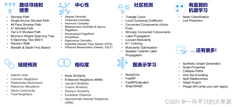
本文继续基于,深入研究基于图谱的各类算法,相比传统的关键词搜索,关系连接,全文检索等,基于知识图谱的算法将充分利用知识图谱的实体关系及其属性权重等信息,为大数据分析做支撑,使得数据分析和知识洞察更直观,可解释和快速解决应用诉求,并可快速落地实施。基于知识图谱的图算法主要有中心度,路径搜索、社区发现,link检测、相似分析和图表示等,详见下图。
另外,在neo4j 4.0之后,不再支持algo了,推出了graph data science(即gds),区别于algo算法库,gds需要根据知识图谱先创建投影图形,投影图的目的是用一个自定义的名称存储在图形目录中,使用该名称,可以被库中的任何算法多次重复引用。这使得多个算法可以使用相同的投影图,而不必在每个算法运行时都对其进行投影。同时,本地投影通过从neo4j存储文件中读取构建,提供了最佳的性能。建议在开发和生产阶段都使用。
如果大家觉得有帮助,欢迎关注并推荐,谢谢啦!
示例实验环境:
neo4 5.1.0,linux7.5,jdk19,plugin有apoc5.1.0、gds2.2.5等。
中心度算法用于识别图中特定节点的角色及其对网络的影响。
######################################################
投影图脚本
1.创建投影图
单个节点,一种关系
call gds.graph.project(

    'mygraph4',

    'com_aaa',

    'has_key',

    {

        relationshipproperties: 'cost'

    }

)
两个节点,两种关系。
call gds.graph.project(

  'mygraph4',

  ['com_aaa', 'result'],

  ['has_key', 'has_key']

)
2.查看投影图是否存在
call gds.graph.exists('mygraph4')

  yield graphname, exists

return graphname, exists
3.删除投影图
call gds.graph.drop('mygraph4') yield graphname;#######################################################
一、实战案例
1.创建投影图,如多个标签和关系的投影
单个节点,一种关系。
call gds.graph.project(

  'mygraph4',

  'com_aaa',

  'has_key'

)
两个节点,两种关系。
call gds.graph.project(

  'wellresult',

  ['com_aaa', 'result'],

  ['has_key', 'has_key']

)
2.pagerank算法
指定一个特定的节点或起点,重点关注这个指定节点的中心度。pagerank算法最初是谷歌推出用来计算网页排名的,简单的说就是,指向这个节点的关系越多,那么这个节点就越重要。
match (source:com_well {name: 'com_aaa'})

call gds.pagerank.stream('wellresult',{ maxiterations: 20, dampingfactor: 0.85, sourcenodes: [source] })

yield nodeid, score

return gds.util.asnode(nodeid) limit 100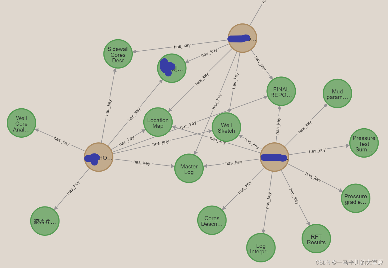
3.shortestpath算法
问题:aaa节点的最短路径(蓝色节点),用于发现源节点和目标节点之间的最短通行路径。
match (source:com_aaa{name: 'aaa'}), (target:result)

call gds.shortestpath.dijkstra.stream('wellresult', {

    sourcenode: source,

    targetnode: target

})

yield index, sourcenode, targetnode, totalcost, nodeids, costs, path

return

    index,

    gds.util.asnode(sourcenode).name as sourcenodename,

    gds.util.asnode(targetnode).name as targetnodename,

    totalcost,

    [nodeid in nodeids | gds.util.asnode(nodeid).name] as nodenames,

    costs,

    nodes(path) as path

order by index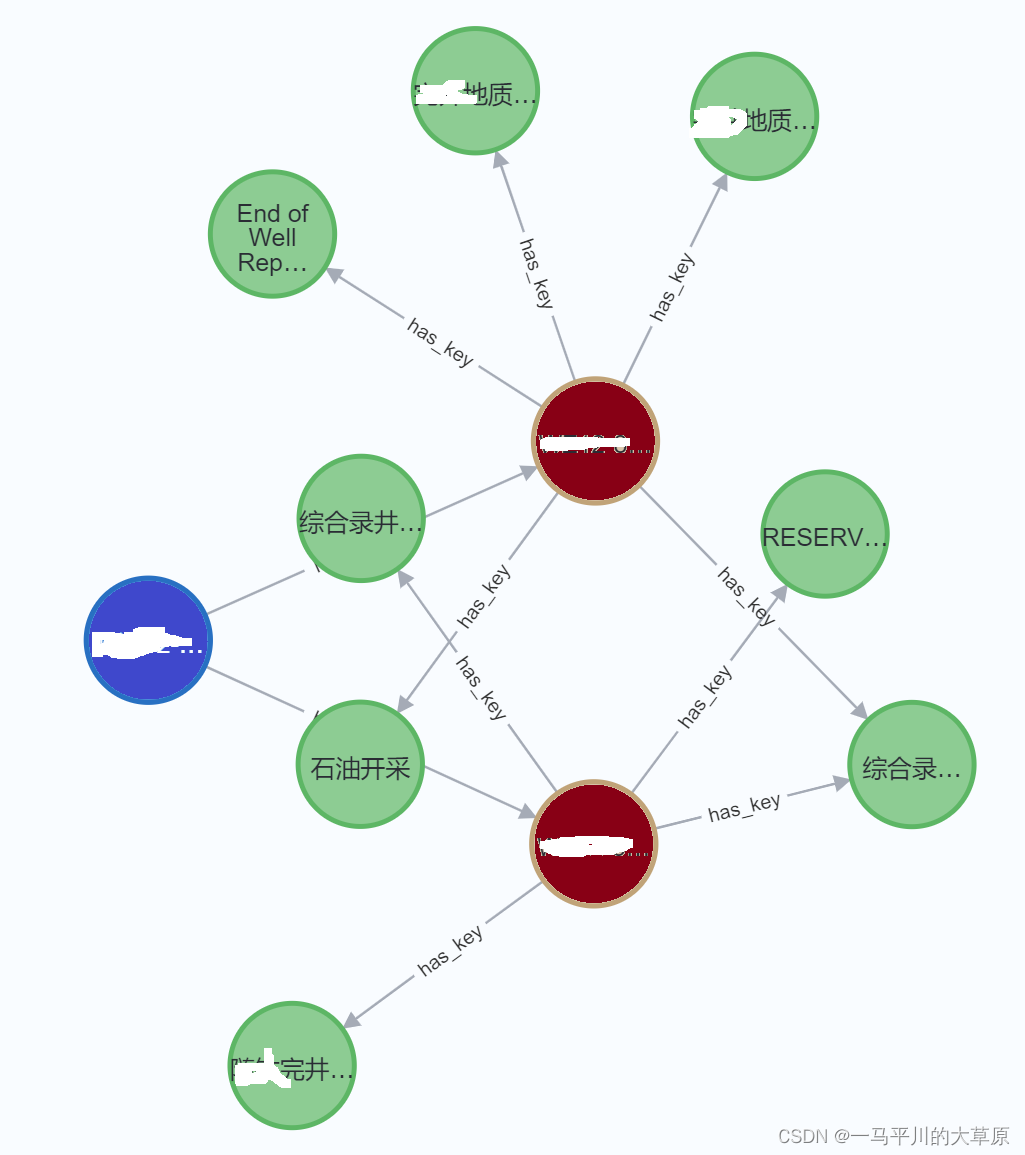
4.allshortestpaths:所有最短路径的集合。
match (source:com_aaa{name: 'xxx'}), (target:result)

call gds.allshortestpaths.delta.stream('wellresult', {

    sourcenode: source,

    delta: 3.0

})

yield index, sourcenode, targetnode, totalcost, nodeids, costs, path

return

    index,

    gds.util.asnode(sourcenode).name as sourcenodename,

    gds.util.asnode(targetnode).name as targetnodename,

    totalcost,

    [nodeid in nodeids | gds.util.asnode(nodeid).name] as nodenames,

    costs,

    nodes(path) as path

order by index
5.深度优先算法(dfs)和广度优先算法(bfs)
快速遍历xxx节点的相关数据。(蓝色节点)
match (source:com_aaa{name: 'xxx'})

call gds.dfs.stream('wellresult', {

  sourcenode: source

})

yield path

return path 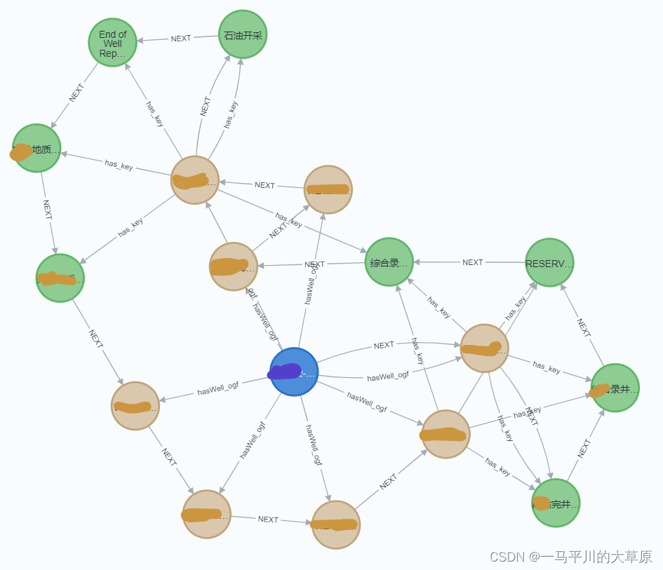
6.随机遍历(randomwalk)
指定节点
match (page:com_aaa)

where page.name in ['aa-1-1']

with collect(page) as sourcenodes

call gds.randomwalk.stream(

  'wellresult',

  {

    sourcenodes: sourcenodes,

    walklength: 3,

    walkspernode: 1,

    randomseed: 42,

    concurrency: 1

  }

)

yield nodeids, path

return nodeids, [node in nodes(path) | node.name ] as pages

match (page:com_aaa)

where page.name in ['aaa']

with collect(page) as sourcenodes

call gds.randomwalk.stream(

  'miningresult',

  {

    sourcenodes: sourcenodes,

    walklength: 3,

    walkspernode: 1,

    randomseed: 42,

    concurrency: 1

  }

)

yield nodeids, path

return nodeids, path limit 100
未指定节点
call gds.randomwalk.stream(

  'wellresult',

  {

    walklength: 3,

    walkspernode: 1,

    randomseed: 42,

    concurrency: 1

  }

)

yield nodeids, path

return nodeids, path limit 20
7.向量化(embeding)
1).node2vec是一种节点嵌入算法,它基于图中的随机行走计算节点的向量表示。邻域是通过随机行走进行采样的。使用一些随机邻域样本,该算法训练了一个单隐层神经网络。该神经网络被训练为根据另一个节点的出现情况来预测一个节点在随机行走中出现的可能性。
2).fastrp快速随机投影,是随机投影算法家族中的一种节点嵌入算法。这些算法在理论上受到johnsson-lindenstrauss定理的支持,根据该定理,人们可以将任意维度的n个向量投影到o(log(n))维度,并且仍然近似地保留各点间的成对距离。事实上,一个以随机方式选择的线性投影满足这一特性。
3).graphsage是一种用于计算节点嵌入的归纳算法。graphsage是利用节点特征信息在未见过的节点或图上生成节点嵌入。该算法不是为每个节点训练单独的嵌入,而是学习一个函数,通过从节点的本地邻域采样和聚集特征来生成嵌入。
call gds.beta.node2vec.stream('wellresult', {embeddingdimension: 4})

yield nodeid, embedding

return gds.util.asnode(nodeid).name, embedding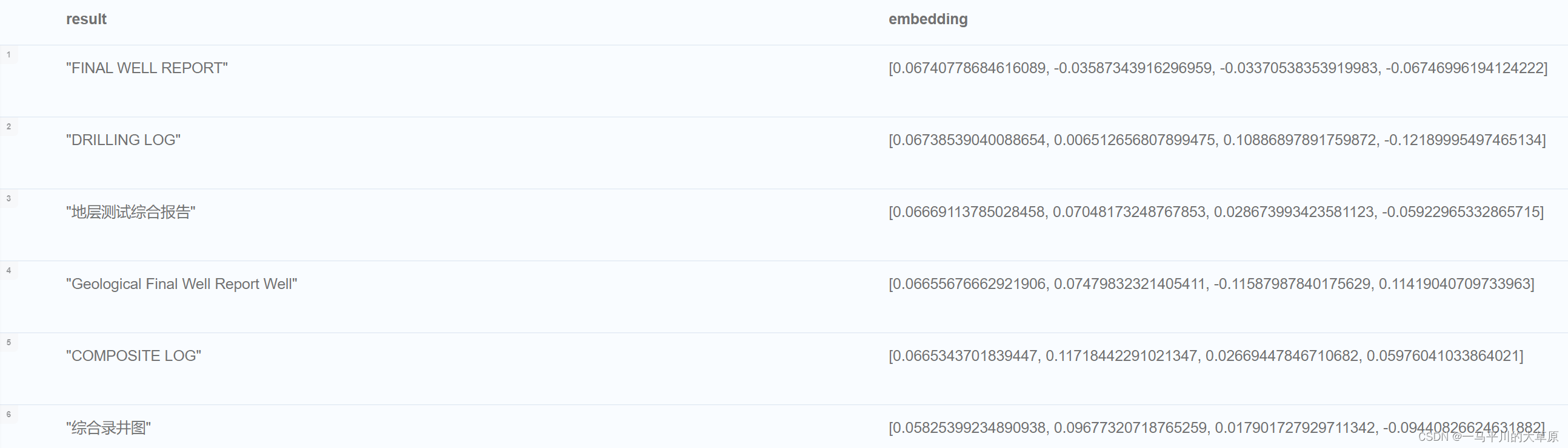
二、参考示例1
数据
merge (home:page {name:"home"})

merge (about:page {name:"about"})

merge (product:page {name:"product"})

merge (links:page {name:"links"})

merge (a:page {name:"site a"})

merge (b:page {name:"site b"})

merge (c:page {name:"site c"})

merge (d:page {name:"site d"})

merge (home)-[:links]->(about)

merge (about)-[:links]->(home)

merge (product)-[:links]->(home)

merge (home)-[:links]->(product)

merge (links)-[:links]->(home)

merge (home)-[:links]->(links)

merge (links)-[:links]->(a)

merge (a)-[:links]->(home)

merge (links)-[:links]->(b)

merge (b)-[:links]->(home)

merge (links)-[:links]->(c)

merge (c)-[:links]->(home)

merge (links)-[:links]->(d)

merge (d)-[:links]->(home)
1.创建投影图
call gds.graph.project(

  'mygraph',

  'page',

  'links',

  {

    relationshipproperties: 'weight'

  }

)
2.计算运行该算法的成本:主要是内存占用成本等
call gds.pagerank.write.estimate('mygraph', {

  writeproperty: 'pagerank',

  maxiterations: 20,

  dampingfactor: 0.85

})

yield nodecount, relationshipcount, bytesmin, bytesmax, requiredmemory
3.pagerank算法
指定一个特定的起点,重点关注这个指定点的中心度
match (sitea:page {name: 'site a'})

call gds.pagerank.stream('mygraph')

yield nodeid, score

return gds.util.asnode(nodeid), score

order by score desc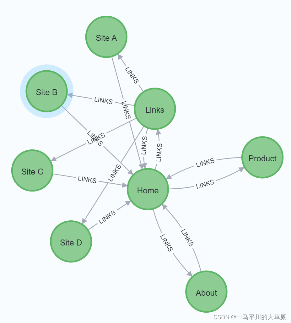
4.randomwalk
call gds.graph.project( 'mygraph2', 'page', { links: { orientation: 'undirected' } } );
未指定源(sourcenodes)

call gds.randomwalk.stream(

  'mygraph',

  {

    walklength: 3,

    walkspernode: 1,

    randomseed: 42,

    concurrency: 1

  }

)

yield nodeids, path

return nodeids, [node in nodes(path) | node.name ] as pages

指定源(sourcenodes)

match (page:page)

where page.name in ['home', 'about']

with collect(page) as sourcenodes

call gds.randomwalk.stream(

  'mygraph',

  {

    sourcenodes: sourcenodes,

    walklength: 3,

    walkspernode: 1,

    randomseed: 42,

    concurrency: 1

  }

)

yield nodeids, path

return nodeids, [node in nodes(path) | node.name ] as pages
统计成本
call gds.randomwalk.stats( 'mygraph', { walklength: 3, walkspernode: 1, randomseed: 42, concurrency: 1 } )
三、参考示例2
数据
create (a:location {name: 'a'}),

       (b:location {name: 'b'}),

       (c:location {name: 'c'}),

       (d:location {name: 'd'}),

       (e:location {name: 'e'}),

       (f:location {name: 'f'}),

       (a)-[:road {cost: 50}]->(b),

       (a)-[:road {cost: 50}]->(c),

       (a)-[:road {cost: 100}]->(d),

       (b)-[:road {cost: 40}]->(d),

       (c)-[:road {cost: 40}]->(d),

       (c)-[:road {cost: 80}]->(e),

       (d)-[:road {cost: 30}]->(e),

       (d)-[:road {cost: 80}]->(f),

       (e)-[:road {cost: 40}]->(f);
1.创建投影图
call gds.graph.project(

    'mygraph',

    'location',

    'road',

    {

        relationshipproperties: 'cost'

    }

)
2.计算运行成本
match (source:location {name: 'a'}), (target:location {name: 'f'})

call gds.shortestpath.dijkstra.write.estimate('mygraph', {

    sourcenode: source,

    targetnode: target,

    relationshipweightproperty: 'cost',

    writerelationshiptype: 'path'

})

yield nodecount, relationshipcount, bytesmin, bytesmax, requiredmemory

return nodecount, relationshipcount, bytesmin, bytesmax, requiredmemory
3.shortestpath算法
match (source:location {name: 'a'}), (target:location {name: 'f'})

call gds.shortestpath.dijkstra.stream('mygraph', {

    sourcenode: source,

    targetnode: target,

    relationshipweightproperty: 'cost'

})

yield index, sourcenode, targetnode, totalcost, nodeids, costs, path

return

    index,

    gds.util.asnode(sourcenode).name as sourcenodename,

    gds.util.asnode(targetnode).name as targetnodename,

    totalcost,

    [nodeid in nodeids | gds.util.asnode(nodeid).name] as nodenames,

    costs,

    nodes(path) as path

order by index
四、参考示例3
数据
create (alice:people{name: 'alice'})

create (bob:people{name: 'bob'})

create (carol:people{name: 'carol'})

create (dave:people{name: 'dave'})

create (eve:people{name: 'eve'})

create (guitar:instrument {name: 'guitar'})

create (synth:instrument {name: 'synthesizer'})

create (bongos:instrument {name: 'bongos'})

create (trumpet:instrument {name: 'trumpet'})

create (alice)-[:likes]->(guitar)

create (alice)-[:likes]->(synth)

create (alice)-[:likes]->(bongos)

create (bob)-[:likes]->(guitar)

create (bob)-[:likes]->(synth)

create (carol)-[:likes]->(bongos)

create (dave)-[:likes]->(guitar)

create (dave)-[:likes]->(synth)

create (dave)-[:likes]->(bongos);
1.投影图
call gds.graph.project('mygraph2', ['people', 'instrument'], 'likes');
2.node2vec向量化
call gds.beta.node2vec.stream('mygraph2', {embeddingdimension: 4})

yield nodeid, embedding

return gds.util.asnode(nodeid).name, embedding

发表评论