【ESP32】手势识别实现笔记：红外温度阵列 | 双三次插值 | 神经网络 | TensorFlow | ESP-DL

开发板：esp32-s3-devkitc-1（esp32-s3-wroom-1-n16r8模块）
开发软件：vs code(espressif idf插件) + anaconda3 + pycharm
开发框架：esp-idf (版本v5.0.4)
训练框架：tensorflow 2.1.0
部署框架：esp-dl
💡💡💡💡： 在stm32上跑神经网络做手势识别 🚀

📍说明：

• 不同手势姿态之间需要具有明显的不同，在使用过程中，手势姿态需要做到位；（可能数据集不足）
• 影响体表温度的因素比较多，由于影响因素的变化，存在部分位置接近环境温度情况，所以即使加入了数据标准化，依然存在推理不准问题；（可能数据集不足）
• 在使用测试中，某个动作出现判断出错，可以将该动作添加到数据集中，在上一次权重文件基础上再训练，修修补补；
• 距离传感器较远，细节难以捕捉，不同手势差异较小，已经无法通过增加数据集来提高预测正确率；
• 该数据集动作主要在中心位置，所以使用过程中动作保持在中心；
• 本示例通过分类任务实现手势识别，如果出现新的手势类别，预测结果就很迷，采用rnn、lstm等的方式，使用效果应该会较好。

一、开发环境搭建与新建工程模板

1.1、开发环境搭建与卸载

考虑 esp-dl 库所支持的版本为 esp-idf v5.0，所以这里安装的不是最新版本。

在安装 vs code插件 (espressif idf) 后，可以选择两种安装方式：

• 在线安装+自动配置 🚀
• 离线安装+手动配置 🚀 （该教程使用的编译操作为 cmd 的方式）

这里采用离线安装+手动配置（vs code下完成程序编辑和编译操作） 💡。

---

① esp-idf 开发环境搭建：

1. 下载esp-idf离线版本：esp-idf windows installer download 🚀
2. 离线安装 esp-idf，安装完成后，安装路径下有三个重要的目录；
   • frameworks/esp-idf-v5.0.4：内含示例代码和组件源代码等；
   • tools：编译器等程序；
   • python_env/idf5.0_py3.11_env：python虚拟运行环境，内含python.exe、pip.exe以及依赖的库等。
3. 打开 vs code，安装插件 espressif idf;
4. vs code 手动配置；
   a) 打开vscode左侧的插件管理页 => 找到espressif idf => 点击该插件旁边的小齿轮 => 扩展设置，就能看到 esp-idf 的配置属性；
   b) 将路径信息添加到这些变量中：custom extra paths、custom extra vars、esp idf path win、esp idf path win、git path、python bin path、tools path win；（参考：esp32 开发环境：windows10 + esp-idf v4.4 + vscode + 插件 espressif idf 搭建踩坑 🚀）
5. 重启一下vs code。

② 打开一个example进行测试：

1. 按住ctrl+shift+p打开命令行，这里输入esp-idf show ，点击 esp-idf: show eaxmples projects，点击需要使用的 esp-idf 路径；
2. 左边栏中选择 hello word 工程，点击 create project using example hello_world。

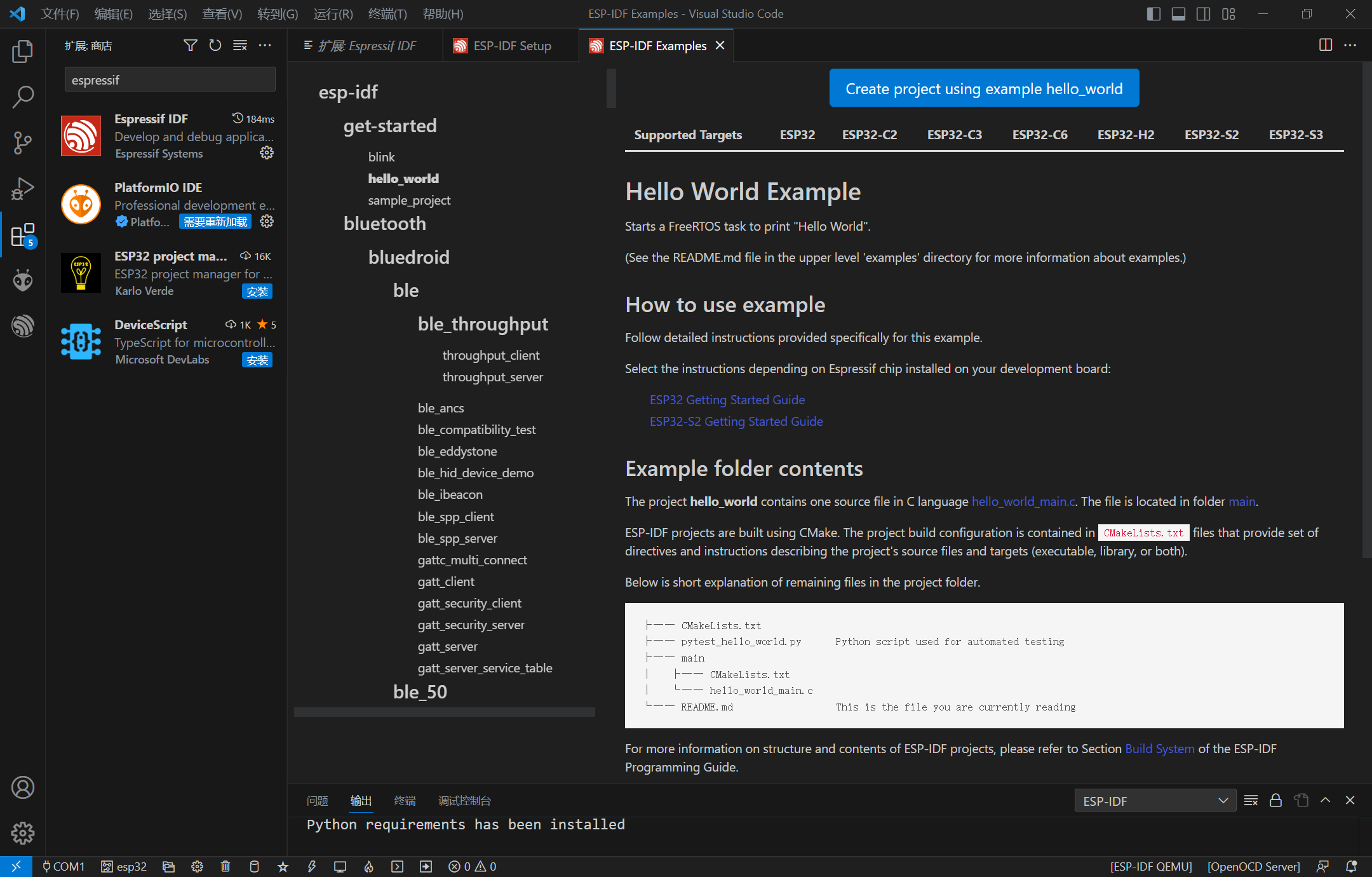
3. 选择这个项目的保存路径，任意路径均可；
4. 烧录过程配置；

5. 点击编译，成功后就可以进行烧录了。

③ 卸载esp-idf： 控制面板 => 卸载程序 => esp-idf tools offline 5.0.4 右键卸载。（vs code 下的配置直接重置就好）

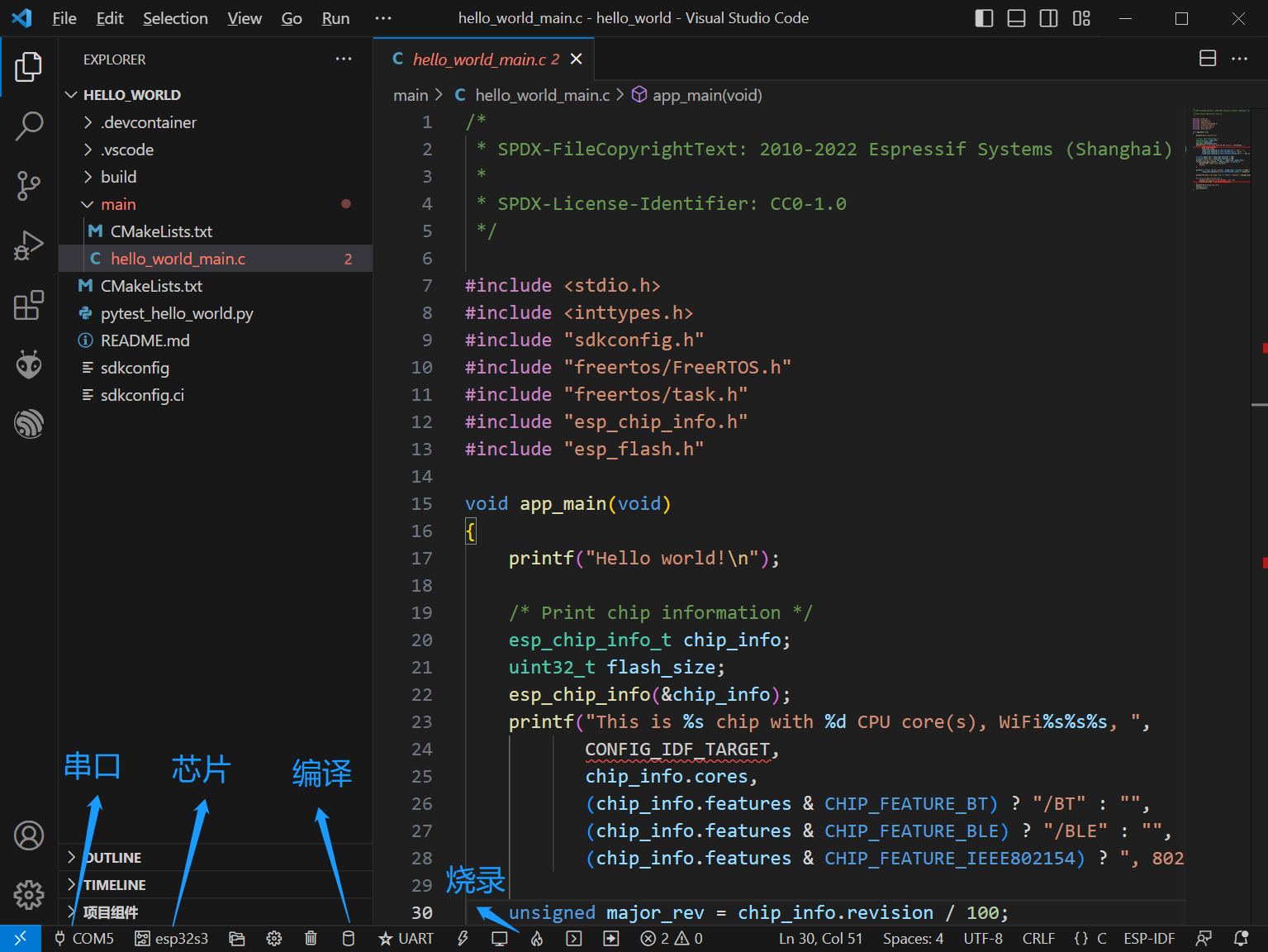
1.2、新建工程目录

1. 打开vs code，此时界面可能是很干净，没有打开项目；这里需要随便打开一个目录（不然第二步操作完发现没响应）；
2. 按住ctrl+shift+p打开命令行，输入esp-idf: create project from extension template，点击；然后就按照提示操作就可以了；
3. 选择项目保存目录；
4. 这里选择template-app，接着就弹出了一个新的vs code界面，关掉前一个vs code界面；
5. 这时候指定目录下就有一个生成的文件夹，修改文件夹名称，方便以后管理（该操作不影响编译）；
6. 打开该目录根目录下的 cmakelists.txt，将 project(template-app) 修改为 project(xxx)，这样之后生成的可执行文件的名称就是xxx.bin，而不是 template-app.bin。点击一下编译查看是否有问题。

1.3、自定义组件

到这一步就可以开发了，为了项目条理更加清晰，还需要引入【自定义组件】。

1. 打开 esp-idf 5.0 cmd 终端，切换到待创建的目录，输入idf.py -c components create-component led；（当然可以手动创建目录和文件）

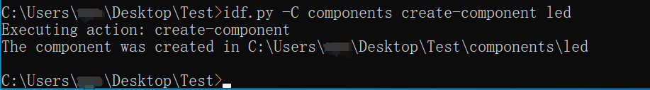
生成后项目目录树如下：

---test
    |---.devcontainer
    |---.vscode
    |---build
    |---cmakelists.txt
    |---sdkconfig
    |---components
            |---led
                 |---include
                        |---led.h
                 |---cmakelists.txt
                 |---led.c
            |---key
                 |---include
                        |---key.h
                 |---cmakelists.txt
                 |---key.c
     |---main
           |---cmakelists.txt
           |---main.c

2. 将组件中的头文件添加到main.c中，这样就可以进行编译了。

3. 如果led组件需要key组件的函数，则：

   • led.h 中加入 #include "key.h"
   • 方式一：led 组件中的 cmakelists.txt 中加入头文件路径：include_dirs "include" "../key/include"（注意这里可是没指定链接路径，但还是能找到）
   • 方式二：led 组件中的 cmakelists.txt 中加入依赖组件：requires driver key（这里led依赖两个组件：driver和key）

4. 在 idf 5.0 的版本之后，driver 组件不作为公共依赖项，所以使用的时候，必须在 cmakelists.txt 中声明依赖 driver 组件后才能使用：

idf_component_register(srcs "led.c"
                    include_dirs "include"
                    requires driver)

参考：
[1]: esp-idf编程指南 🚀
[2]: esp—idf开发（1）创建模板工程 🚀
[3]: esp32学习笔记（21）——构建自己的工程和组件库 🚀
[4]: esp32 esp-idf自定义组件 🚀
[5]: esp32开发 cmakelists包含同级目录.h文件，error: gpiox.h: no such file or directory 🚀

二、驱动移植与应用开发

管脚布局：

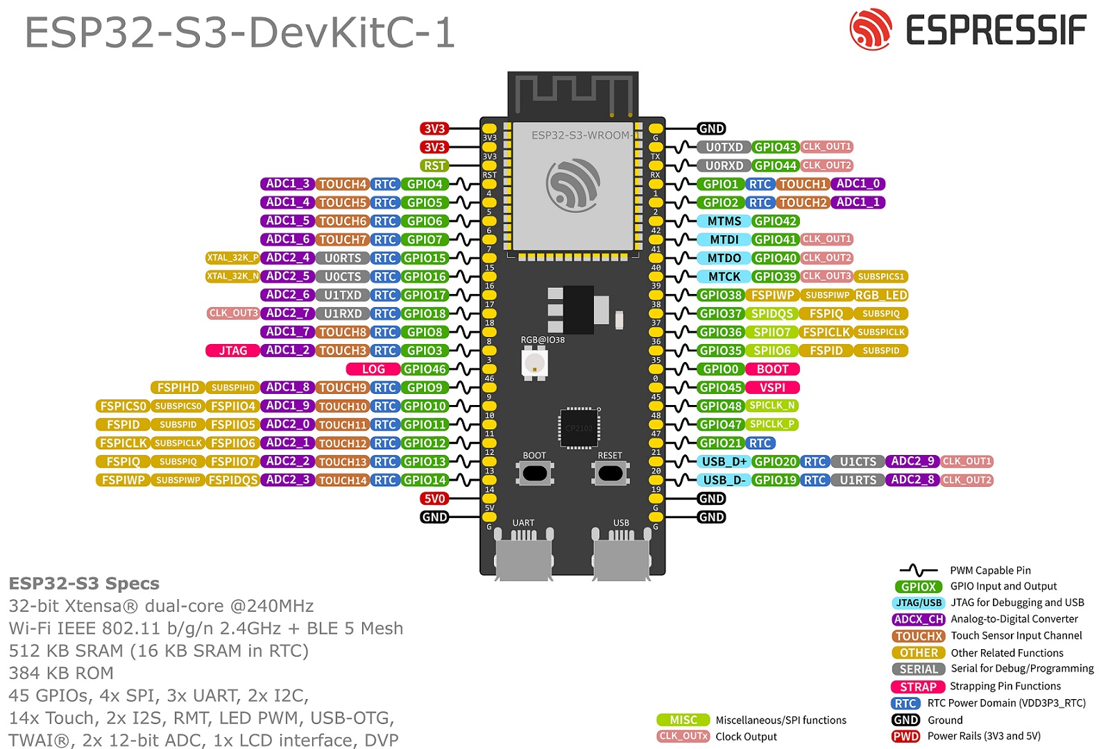
i2c0引脚资源使用情况： 支持任意 gpio 管脚

  ------------------------------------
  |   amg8833       |   esp32        |
  ------------------------------------
  |   vin           |   3.3v         |
  |   gnd           |   gnd          |
  |   scl           |   gpio2        |
  |   sda           |   gpio1        |
  |   int           |   /            |
  |   ad0           |   gnd          |  
  ------------------------------------

spi3引脚资源使用情况： 支持任意 gpio 管脚

  ------------------------------------
  |  lcd screen     |   esp32        |
  ------------------------------------
  |  gnd            |   gnd          |
  |  vcc            |   vcc(3.3v)    |
  |  scl            |   gpio5(sclk)  |
  |  sda            |   gpio6(mosi)  |
  |  res            |   gpio7        |
  |  dc             |   gpio15       |
  |  cs             |   gpio16       |
  |  blk            |   gpio17       |
  ------------------------------------

2.1、i2c驱动移植与amg8833应用开发

esp32-s3 有2个 i2c 控制器，每个控制器都可以设置为主机或从机，本次示例中作为主机使用。

• 当 8x8 中某个测点出现超过极限值就会触发int引脚电平变化，esp32 通过 int 引脚触发外部中断；esp32 通过读取寄存器的值就可以确定哪个矩阵测点触发电平变化。
• amg8833 scl最大支持 400khz。
• ad0（ad_select）为 i2c设备地址选择脚。拉低，设备地址为110 1000，即0x68。拉高，设备地址为110 1001，即0x69。
• eps32-s3 的 i2c 引脚原则上可选择任意引脚，在 i2c 初始化的时候指定即可，并将引脚设置为 enable gpio pull-up resistor。

主机写入数据：

1. 使用 i2c_cmd_link_create() 创建一个命令链接。然后，将一系列待发送给从机的数据填充命令链接：
   a. 启动位 - i2c_master_start()
   b. 从机地址 - i2c_master_write_byte()。提供单字节地址作为调用此函数的实参。
   c. 数据 - 一个或多个字节的数据作为 i2c_master_write() 的实参。
2. 通过调用 i2c_master_cmd_begin() 来触发 i2c 控制器执行命令链接。一旦开始执行，就不能再修改命令链接。（一般报错出现在该语句）
3. 命令发送后，通过调用 i2c_cmd_link_delete() 释放命令链接使用的资源。
   

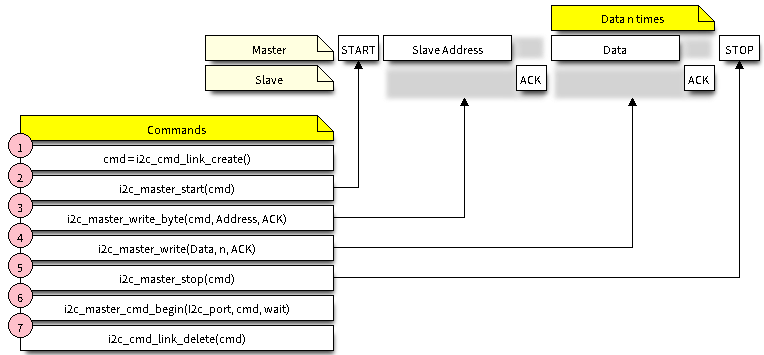
主机读取数据的步骤基本相似。

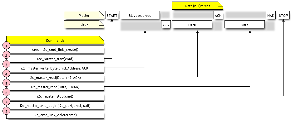
esp-idf 对这两个过程进行了封装：

• 主机读取数据：i2c_master_write_read_device()
• 主机写入数据： i2c_master_write_to_device()

基本过程同上面一致，本示例依据这两个函数源代码，进行简单修改。

amg8833 需要进行初始化寄存器：正常读取前需要进行初始化操作。

• power control寄存器：设置amg8833的工作模式；
• reset寄存器：进行软复位；
• frame rate寄存器：设定帧率；
• interrupt control寄存器：配置中断功能；

amg8833 temperature寄存器：红外点阵测量的温度值。

两个寄存器的数据组合起来获得一个测点的温度值。有12位数据，最高位为符号位，0为正，1为负。最小变化单位为0.25℃。

在读取64个像素点温度值时候，i2c只需要指定第一个寄存器地址以及读取的字节数量，amg8833自动发送后面地址的数据。

/* arduino框架下测试代码, 用于对比在esp-idf框架下驱动与应用是否正常
 * 这里在测试代码的基础上增加/修改了两条语句:
 * => wire.setpins(1,2); // 设置新的i2c引脚
 * => status = amg.begin(0x68, &wire); //amg8833初始化, 0x68为amg8833设备地址
*/

#include <wire.h>
#include <adafruit_amg88xx.h>

adafruit_amg88xx amg;

float pixels[amg88xx_pixel_array_size];

void setup() {
    serial.begin(9600);
    serial.println(f("amg88xx pixels"));

    bool status;
    wire.setpins(1,2); //new sda scl pins
    // default settings
    status = amg.begin(0x68, &wire);
    if (!status) {
        serial.println("could not find a valid amg88xx sensor, check wiring!");
        while (1);
    }
    
    serial.println("-- pixels test --");

    serial.println();

    delay(100); // let sensor boot up
}


void loop() { 
    //read all the pixels
    amg.readpixels(pixels);

    serial.print("[");
    for(int i=1; i<=amg88xx_pixel_array_size; i++){
      serial.print(pixels[i-1]);
      serial.print(", ");
      if( i%8 == 0 ) serial.println();
    }
    serial.println("]");
    serial.println();

    //delay a second
    delay(1000);
}

参考：
[1]: esp_idf—i2c 驱动程序 🚀
[2]: esp32 之 esp-idf 教学（六）——硬件i2c总线外设（i²c） 🚀
[3]: amg8833的使用与stm32驱动代码 🚀
[4]: esp32 i2c自定义引脚 🚀
[5]: esp32-s3入门arduino开发（一）–arduino环境搭建 🚀

2.2、spi驱动移植与lcd应用开发

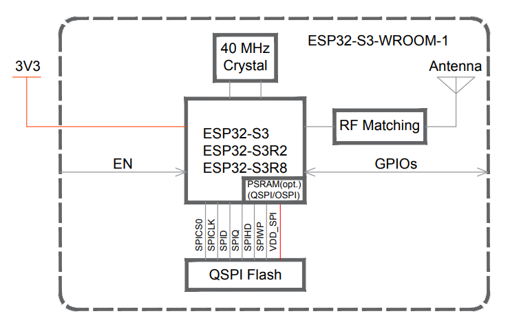
esp32-s3-devkitc-1 开发板采用 esp32-s3-wroom-1/1u 或 esp32-s3-wroom-2/2u 模组，而这些模组采用 esp32-s3芯片。

esp32-s3 芯片集成了四个 spi 控制器：

• spi0
• spi1
• 通用 spi2，即gp-spi2
• 通用 spi3，即gp-spi3

spi0 和 spi1 控制器主要供内部使用以访问外部 flash 及 psram，如上图所示。这里采用 spi3 作为 lcd 通信控制器。

spi有多种模式：为兼容lcd通信规范，这里采用普通 spi 模式。

• 普通 spi 模式
• 双线输出模式
• 双线输出模式
• 四线输出模式
• 四线 i/o 模式
• 八线输出模式
• opi 模式

lcd驱动和应用编写：

1. spi初始化：引脚指定、频率、最大传输数据大小、是否开启dma等，主要配置 spi_bus_config_t 和 spi_device_interface_config_t 结构体；通过 spi_bus_initialize 和 spi_bus_add_device 函数完成配置；

2. 普通gpio初始化：dc、rst、bck引脚不在spi协议所规定的引脚，所以需要单独进行初始化；

3. 编写命令/数据spi发送函数；
4. 编写lcd初始化；
5. 编写矩形绘制和图片显示函数，验证程序工作正常。

参考：
[1]: esp32-idf开发笔记 | 03 - 使用spi外设驱动st7789 spilcd 🚀
[2]: 【esp32-idf】 02-4 外设-spi 🚀
[3]: esp-idf 编程指南：spi 主机驱动程序 🚀

2.3、绘制温度云图

camcolors全局变量数组，里面保存颜色数据（rgb565），共有256种颜色，0索引保存为蓝色，255索引保存为红色。

最大温度记作：$t_{max}$；最小温度记作：$t_{min}$；当前温度记作：$t_{cur}$。
最小索引值记作：$idx$。

建立温度和颜色的映射关系：

$$\frac{t_{max}-t_{min}}{255-0}=\frac{t_{cur}-t_{min}}{x-0}$$

转换为：

$$x=255\ast \frac{t_{cur}-t_{min}}{t_{max}-t_{min}}$$

arduino 框架官方提供了映射函数——map函数，主题思想一致的，细节上有些差异，具体表示如下：

$$x=\frac{255\ast (t_{cur}-t_{min})+(t_{max}-t_{min})/2}{t_{max}-t_{min}}+idx=255\ast \frac{t_{cur}-t_{min}}{t_{max}-t_{min}}+0.5+idx$$

浮点型赋值给整型，小数部分舍去，这里加上0.5，实现四舍五入。

2.4、启用psram（可选）

1. 点击齿轮
   
2. 输入 ram查找一下两项，勾选support for external, spi-connected ram以及模式选择octal mode psram。
   
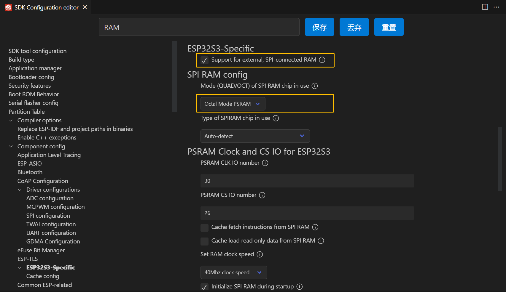
3. 选择make ram alloctable using heap_caps_malloc(...,malloc_cap_spiram)，也可以选择make ram allocatable using malloc() as well，之所以选择前者是从存储器的使用上考虑：若从片上 sram 分配空间，则使用malloc函数，若从片外 psram 上分配空间，则使用heap_caps_malloc函数。
   
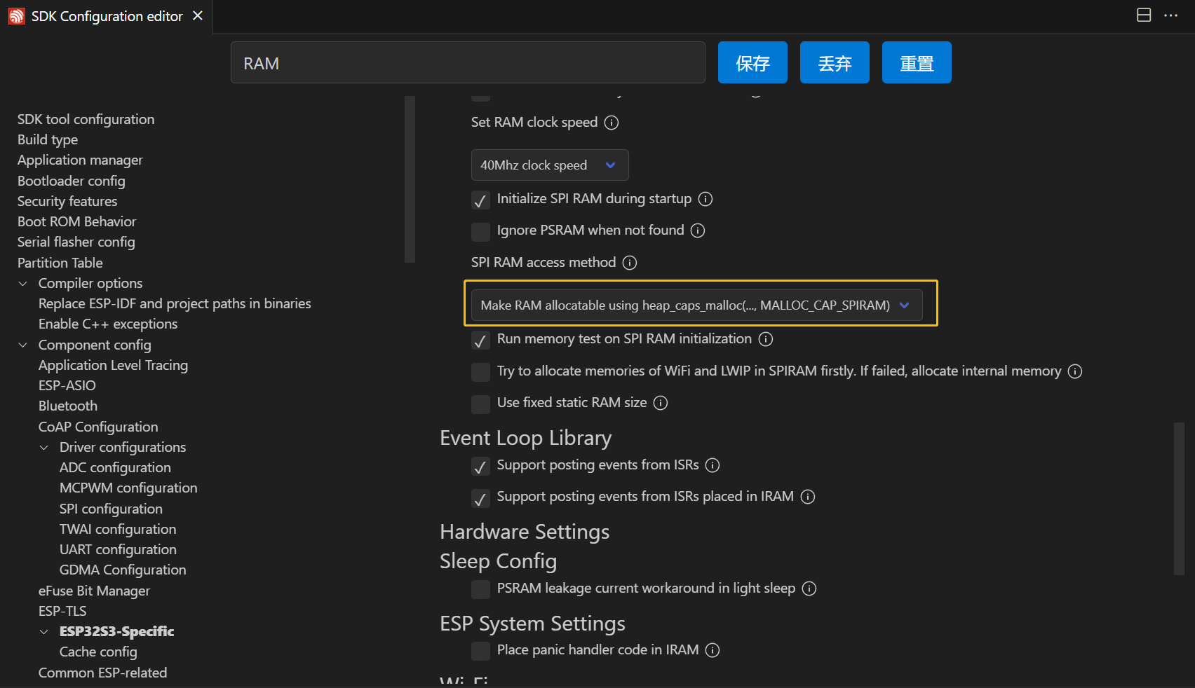
4. 其它参数可使用默认。
5. 保存，然后编译。

2.5、画面动静和距离检测

这里画面动静判断采用帧间差分法，以目标温度较小值为分界点，区分背景和目标，将两帧温度矩阵（24x24）的对应点进行相减，并取其绝对值，若大于阈值（目标和背景采用不同阈值）则计数值加1，当计数值大于某个值（距离不同，检测到目标的大小也不同，这个值是实时调整）后，则认为画面中存在运动目标。

在实现过程中，由于对比两帧数据，所以需要保存前一帧温度矩阵数据，一帧数据大小为24x24x4(float) = 2.25kb，这里采用 异步内存拷贝(asynchronous memory copy)，其核心技术在于dma，通过给dma发送命令，实现内存拷贝，此时不需要cpu参与，当传输完成后通过回调函数发送信号通知被阻塞的任务。

异步内存拷贝：

/*-------------------> 安装 <-------------------*/
config = async_memcpy_default_config();
config.backlog = 16; // update the maximum data stream supported by underlying dma engine
async_memcpy_t mem_driver = null;
esp_error_check(esp_async_memcpy_install(&config, &mem_driver)); // install driver with default dma engine

semaphorehandle_t my_semphr = xsemaphorecreatebinary(); // create a semaphore used to report the completion of async memcpy


/*--------------> 发送内存拷贝请求 <--------------*/
esp_error_check(esp_async_memcpy(mem_driver, out_img_buf_pre, out_img_buf, copy_len, my_async_memcpy_cb, &myflags));

/*-----------> 拷贝完成后调用回调函数 <-----------*/
// callback function, running in isr context
static bool my_async_memcpy_cb(async_memcpy_t mcp_hdl, async_memcpy_event_t *event, void *cb_args)
{
    /*可自定义标志*/
    
    basetype_t high_task_wakeup = pdfalse;
    xsemaphoregivefromisr(my_semphr, &high_task_wakeup); // high_task_wakeup set to pdtrue if some high priority task unblocked
    return high_task_wakeup == pdtrue;
}

/*-----------> 阻塞等待内存拷贝完成 <-----------*/
xsemaphoretake(my_semphr, portmax_delay); // wait until the buffer copy is done

画面动静判断逻辑：

//获取第一帧24x24温度矩阵
readpixels{}
//保存第一帧数据
mem2mem{
	1.发送内存拷贝请求
	2.sigflag = 1
}

while(1){
	readpixels{} //获取24x24温度矩阵
	motion_detection{
		if(sigflag == 1){
			1.阻塞等待内存拷贝完成
			2.sigflag == 0
		}
		
		/*画面动静判断*/
		
		if(运动){
			mem2mem{} // 如果运动, 保存当前帧数据
		}
		else{ // 静止, 不保存数据
		}
	}
}

1. 获取第一帧24x24温度矩阵；
2. 保存第一帧数据；
3. 获取第二帧24x24温度矩阵；
4. 因为是第一帧，所以等待第一帧保存完成；
5. 判断是否运动，若为运动，保存当前帧(第二帧)，下一次和第二帧做比较，若为静止，不用保存，下一次和第一帧做比较；
6. 开始第二次循环，获取第三帧24x24温度矩阵；
7. 是否之前有保存操作，没有就不用阻塞等待，有就阻塞等待；
8. 判断是否运动，继续循环往复。

参考：
[1]: 运动目标检测——帧间差分法(temporal difference)简介 🚀
[2]: 🚀
[3]: the async memcpy api 🚀

---

目标距离检测实现原理：靠近传感器温度高，远离传感器温度低。

这种方式存在一个问题：如果目标远离检测范围那么温度也会下降，进入检测范围那么温度也会上升，更复杂是前后左右平移+上下平移的复合动作，这里暂时不考虑，只考虑上下平移。🔍

2.6、图像放大之双三次插值法：权重计算 | 插值计算 | 程序设计

对于低分辨图像在高分辨率的设备上显示，如果不做任何处理，那么实际显示区域会很小，为了扩大显示区域，就需要对低分辨率的图像进行数值图像放大处理，就是将低分辨率的图像变成高分辨率的图像，多出来的像素怎么获得？—— 插值算法。

虽然变成了高分辨率图像，但是这是由低分辨率的数据生成的，所以不会很高清。

常见的插值算法：自适应和非自适应。
非自适应算法：最近邻，双线性，双三次，样条等。双三次插值效果较好，但是时间开销比较大。

基本步骤：

1. 计算权重
2. 计算放大图像后的像素值

---

1、权重计算

原图片：8x8
放大后的图片：16x16

将【放大后的图片】缩小到【原图片】的大小，如下图所示：

缩小后，每个像素（共16x16个）都需要计算权值。当计算某个像素权值时，取该像素上下左右邻近的四个点，在这四个点为基础，向外再扩充一圈，总共取16个点，如下图所示：

将上面的距离数据代入权重计算公式：

$$w(x)=\{\begin{array}{l}(a+2)|x{|}^3-(a+3)|x{|}^2+1for|x|\le 1\\ a|x{|}^3-5a|x{|}^2+8a|x|-4afor1\le |x|\le 2\\ 0others\end{array}$$

式中，$x$ 为目标像素点距离邻近像素点的距离；$a$ 一般取 $-0.5$。

对于【米黄色】的点，x轴方向距离为0.6，y轴方向距离为1.3。

• x轴方向：
  $$\begin{array}{rl}w(x)& =(a+2)|x{|}^3-(a+3)|x{|}^2+1\\ & =(-0.5+2)\ast |0.6{|}^3-(-0.5+3)\ast |0.6{|}^2+1\\ & =0.424\end{array}$$

• y轴方向：
  $$\begin{array}{rl}w(y)& =a|x{|}^3-5a|x{|}^2+8a|x|-4a\\ & =(-0.5)\ast |1.3{|}^3-5\ast (-0.5)\ast |1.3{|}^2+8\ast (-0.5)\ast |1.3|-4\ast (-0.5)\\ & =-0.0735\end{array}$$

对于【浅绿色】的点，x轴方向距离为1.6，y轴方向距离为1.3。

• x轴方向：
  $$\begin{array}{rl}w(x)& =a|x{|}^3-5a|x{|}^2+8a|x|-4a\\ & =(-0.5)\ast |1.6{|}^3-5\ast (-0.5)\ast |1.6{|}^2+8\ast (-0.5)\ast |1.6|-4\ast (-0.5)\\ & =-0.048\end{array}$$

• y轴方向：
  $$\begin{array}{rl}w(y)& =a|x{|}^3-5a|x{|}^2+8a|x|-4a\\ & =(-0.5)\ast |1.3{|}^3-5\ast (-0.5)\ast |1.3{|}^2+8\ast (-0.5)\ast |1.3|-4\ast (-0.5)\\ & =-0.0735\end{array}$$

每个插值的像素都是由16个原图中像素加权计算所得，每一行x轴方向权重相同，每一列y轴方向权重相同，所以一个插值的像素需要进行8次权重计算。

---

2、插值计算

计算红点位置的像素值，取4x4区域中的16个点。

然后计算原图像素和权重的hadamard积：

最后，将矩阵中所有元素相加得到了插值的像素值。

---

由上图可知：

• 当距离为0的时候，$w=1$
• 当距离为-1或1的时候，$w=0$
• 当距离为-2或2的时候，$w=0$

所以当【放大后的图片】像素点与【原图片】像素点重合的时候，距离绝对值取值可能为0、1和2，那么最后插值计算的结果就是重合原图片像素点。

参考：
[1]: 用于数字成像的双三次插值技术 🚀
[2]: 插值算法 ｜ 双三次插值算法 🚀（视频中a = -0.75）

3、程序设计

按照上述基本原理进行程序实现，具体函数在 gesture_display.cpp 文件中，其中有两个主要接口：

• interpolate_image函数：实现8x8温度值放大成24x24温度值；
• temp_cloud_map_display函数：将温度值通过云图方式在lcd上显示；

+----------------------------------------------------------------------------+
|                                           +-------------------------------+|
| ==> getw_x() ==> weight_xy_adjust2d() ==> | matrix_hadamard_pruduct()     ||
| ==> getw_y() ==> weight_xy_adjust2d() ==> | img_matrix_hadamard_pruduct() ||
| ==> img8x8_pad_to_img12x12() ===========> | matrix_elem_sum()             ||
|                                           +-------------------------------+|                                           
|----------------------------------------------------------------------------|
| *************************   interpolate_image()  ************************* |
+----------------------------------------------------------------------------+

参考：
[1]: 图像的放大：双三次插值算法（c++实现） 🚀

四、数据集获取

上位机程序（pc）：get_data/get_data.py
下位机程序（esp32）：get_data/esp_dl_for_bixin

使用逻辑：

1. lcd显示采集温度云图，若符合要求，按下键盘任意键+回车；
2. 按下后，通过串口发送给esp32，esp32收到命令后，申请互斥锁，阻塞温度采集和插补计算，绘制当前温度云图，确认温度云图是否符合预期；
3. 上位机输入标签或者放弃该数据，若输入数字标签（0-背景，1-放大，2-捏住，3-减小），则将命令发送给esp32，等待esp32将点阵数据发送；若放弃，输入数字4，则将命令发送给esp32，重新进行温度采样；
4. pc设备在收到串口数据后，复原图像，然后根据标签将数据和图片保存到对应目录下，文件名自动加1；（若上位机程序中途退出，下次运行时候，需要将当前的文件数量覆盖num1/num2/num3/num3变量）
5. 然后重新开始第一步。

五、cnn模型训练

5.1、环境配置：anconda3 | tf2.1.0 | pycharm

python：3.7（anaconda3）
开发框架：tensorflow 2.1.0
ide：pycharm

① python安装：

anaconda：python编译器和python包管理工具合在一起的一个软件。

安装配置教程： 🚀

# 虚拟环境常用命令
conda info -e  # 查看已经创建的所有虚拟环境
conda create -n xxx python=3.7  # 创建一个python3.7 名为xxx的虚拟环境
conda activate xxx  # 切换/激活到xx虚拟环境

② tensorflow安装：

// gpu 版本
pip install --upgrade tensorflow-gpu==2.0.0 -i https://pypi.tuna.tsinghua.edu.cn/simple

// cpu 版本
pip install --upgrade tensorflow-cpu==2.1.0 -i https://pypi.tuna.tsinghua.edu.cn/simple

检测是否安装成功：切换到虚拟环境——>输入python ——> 载入tensorflow （import tensorflow as tf） ——> 查看版本号（print(tf.__version__)）

③ pycharm安装：

可以直接从 pycharm 官网下载，但是可能由于 anaconda 版本比较老，添加 python 解释器比较麻烦，所以这里采用这位博主提供的版本，具体软件安装、解释器添加教程可 🚀。

5.2、生成数据集 | 预处理

由第四章中所构建的数据集，*.txt 文件中保存的数据为温度值，数据的排布格式如上所示，将*.txt文件中的数据变成数据集需要考虑以下事情：

• 【生成数据集】保存的数据按照分类分别保存在不同的目录下，所以需要统计数据集目录下所有的数据，将数据打乱，按照60%训练-20%测试-20%验证的比例划分。
• 【预处理】*.txt 文件中的数据类型为字符串，而训练时候所需要的数据为 float。

5.2.1、生成数据集：统计数据集 | 数据集随机化 | 数据集划分

1. 创建数字编码表，即手势行为与数字的对应关系，background=0，increase=1，pinch=2，reduce=3；
2. 遍历文件夹下的所有文件，以列表的方式保存所有文件的路径；
3. 通过 random.shuffle 打乱顺序；
4. 读取列表每个元素值然后拆解，由于原先存放的顺序以类别分别存放在对应的目录下，所以从拆解的结果可以知道该数据对应的标签，将【数据路径(*.txt)】和【标签】保存到 csv 文件中；
5. 从 csv 文件中读出数据，按【数据路径】和【标签】分别保存到两个变量中，返回；
6. 按照比例，以切片的方式，得到训练集、测试集、验证集，注意这里的数据还只是数据的路径，后面输入到神经网络需要将数据提取处出来，这部分工作交给预处理来完成。

目录结构：

---xxx
    |---dataset
           |---background
                   |---1.jpg
                   |---1.txt
                   |---...
           |---increase
                   |---1.jpg
                   |---1.txt
                   |---...
           |---pinch
                   |---1.jpg
                   |---1.txt
                   |---...
           |---reduce
                   |---1.jpg
                   |---1.txt
                   |---...
           |---tmp_data.csv
    |---geture_train.py

代码如下：

# 作用：将文件统计存入csv文件，然后读出csv文件内容
# root:数据集根目录
# filename:csv文件名
# name2label:类别名编码表
def load_csv(root, filename, name2label):
    if not os.path.exists(os.path.join(root, filename)):
        tmp_data = []
        for name in name2label.keys():
            # 'dataset\\increase\\1.txt
            tmp_data += glob.glob(os.path.join(root, name, '*.txt'))

        # 200, 'dataset\increase\\1.txt'...
        print(len(tmp_data), tmp_data)

        random.shuffle(tmp_data)
        with open(os.path.join(root, filename), mode='w', newline='') as f:
            writer = csv.writer(f)
            for img in tmp_data:  # 'dataset\\increase\\1.txt'
                name = img.split(os.sep)[-2]
                label = name2label[name]
                # 'dataset\\increase\\1.png', 1
                writer.writerow([img, label])
            print('written into csv file:', filename)

    # read from csv file
    tmp_data, labels = [], []
    with open(os.path.join(root, filename)) as f:
        reader = csv.reader(f)
        for row in reader:
            # 'dataset\\increase\\1.txt', 1
            tmp, label = row
            label = int(label)

            tmp_data.append(tmp)
            labels.append(label)

    assert len(tmp_data) == len(labels)

    return tmp_data, labels


# root:数据集根目录
def load_gesture(root, mode='train'):
    # 创建数字编码表
    name2label = {}  # "sq...":0
    for name in sorted(os.listdir(os.path.join(root))):
        if not os.path.isdir(os.path.join(root, name)):
            continue
        # 给每个类别编码一个数字
        # 如: name2label['increase'] = 1
        name2label[name] = len(name2label.keys())

    print(name2label)

    # 读取label信息
    # [file1,file2,], [3,1]
    images, labels = load_csv(root, 'tmp_data.csv', name2label)

    if mode == 'train':  # 60%
        images = images[:int(0.6 * len(images))]
        labels = labels[:int(0.6 * len(labels))]
    elif mode == 'val':  # 20% = 60%->80%
        images = images[int(0.6 * len(images)):int(0.8 * len(images))]
        labels = labels[int(0.6 * len(labels)):int(0.8 * len(labels))]
    else:  # 20% = 80%->100%
        images = images[int(0.8 * len(images)):]
        labels = labels[int(0.8 * len(labels)):]

    return images, labels, name2label

5.2.2、预处理：string类型转换为float | 数据标准化 | one-hot encoding

预处理工作通过map的方式实现，将每个路径的 txt 加载进来替换掉，变成 txt 本身的内容，即 $x$ 由原先路径，变成 [24, 24] 温度矩阵数据，$y$ 为标签数据。

1. 读取 *.txt 中的数据，该数据为一个字符串；
2. 删除字符串中的空格和\r\n字符，然后以这些字符，分割字符串，产生 576 个字符串，以列表的方式保存；
3. 将 576 个字符串转换为 float 类型，此时列表为 576 个 float 类型元素，shape为 [576]；
4. 将 [576] shape 转换为 [24, 24] shape，并进行扩展维度，将 [24, 24] shape 转变为 [24, 24, 1]；
5. 采用最大最小标准化（min-max normalization）：$x^{{}^{\prime }}=\frac{x-min(x)}{max(x)-min(x)}$ （对 $x$ 数据进行标准化处理）；
6. 将 label 数据（$y$）转换为 tensor 类型，并进行 one-hot encoding 处理（共 4 种类型，数字0，编码后变成 [1,0,0,0]）；
7. 导出 $x$ 和 $y$ 两种 tensor 数据。

代码如下：

def preprocess(x, y):  # 这个顺序和from_tensor_slices中的 x,y 对应
    # 读入txt数据
    data = tf.io.read_file(x)

    # 分割每行数据
    data = tf.strings.split(data)  # "22.11 22.11 ...\r\n22.11 22.11...\r\n" => ["22.11" "22.11" ...]
    data = tf.strings.to_number(data)  # ["22.11" "22.11" ...] (string) => [22.11 22.11 ...] (float32)
    data = tf.reshape(data, [24, 24])  # shape [576] => shape [24, 24]
    data = tf.expand_dims(data, axis=2)  # shape [24, 24] => shape [24, 24, 1]

    # data数据归一化
    max_data = tf.reduce_max(data)  # 标量
    min_data = tf.reduce_min(data)  # 标量
    data = (data - min_data)/(max_data-min_data)  # broadcat 张量维度扩张

    y = tf.convert_to_tensor(y)
    y = tf.one_hot(y, depth=4)  # one-hot encoding
    return data, y

5.3、构建训练模型

conv_layers = [
    # kernel_size:3x3, 卷积核个数:4
    layers.conv2d(4, input_shape=(24, 24, 1), kernel_size=[3, 3], padding="valid", activation=tf.nn.relu),  # [b, 24, 24, 1] => [b, 22, 22, 4]
    layers.maxpool2d(pool_size=[2, 2], strides=2, padding='valid'),  # [b, 22, 22, 4] => [b, 11, 11, 4]
    layers.flatten(),  # [b, 11, 11, 4] => [b, 484]
    layers.dense(128, activation=tf.nn.relu),  # [b, 484] => [b, 128]
    layers.dense(64, activation=tf.nn.relu),  # [b, 128] => [b, 64]
    layers.dense(4, activation=tf.nn.softmax),  # [b, 64] => [b, 4]
]

def main():
    print(tf.__version__)
    train_images, train_labels, train_table = load_gesture('.\\dataset', 'train')
    val_images, val_labels, val_table = load_gesture('.\\dataset', 'val')

    train_db = tf.data.dataset.from_tensor_slices((train_images, train_labels))
    train_db = train_db.map(preprocess).batch(300)

    val_db = tf.data.dataset.from_tensor_slices((val_images, val_labels))
    val_db = val_db.map(preprocess).batch(300)

    # [b, 24, 24, 1] => [b, 4]
    network = sequential(conv_layers)

    # network.build(input_shape=[none, 24, 24, 1])
    network.compile(optimizer=optimizers.adam(lr=1e-4), # adam优化器配置
                    loss=tf.losses.categoricalcrossentropy(from_logits=false),  # 损失函数: 交叉熵
                    metrics=['accuracy'])  #  准确率计算

	# 打印网络信息
    network.summary()

	# 模型训练和验证
    network.fit(train_db, epochs=200, validation_data=val_db, validation_freq=1)

构建模型的时候，输入张量设置方式有多种，上面的是直接在模型conv_layers 中添加，或者可以使用model.build(input_shape=[none, 24, 24, 1])，这两种方式存在一定的差异，至少在onnx模型转换的时候，第二种方式会报错：‘sequential’ object has no attribute ‘output_names’；并且二者的ckpt权值文件也是不通用的，提示：shapes (128,) and (64,) are incompatible。

5.4、训练结果保存和准确率

在构建模型的基础上，添加权值保存语句：

checkpoint_path = "gesture_train-{epoch:02d}.ckpt"  # ckpt保存文件名, 占位符将会被epoch值和传入on_epoch_end的logs所填入
cp_callback = tf.keras.callbacks.modelcheckpoint(filepath=checkpoint_path,  # 保存文件名
                                                     save_best_only=true,  # 当设置为true时，将只保存在验证集上性能最好的模型
                                                     save_weights_only=true,  # 若设置为true，则只保存模型权重，否则将保存整个模型（包括模型结构，配置信息等）
                                                     verbose=1,  # 为1表示输出epoch模型保存信息，默认为0表示不输出该信息
                                                     save_freq='epoch'  # checkpoint之间的间隔的epoch数
                                                     )

network.fit(train_db, epochs=200, validation_data=val_db, validation_freq=1, callbacks=[cp_callback])

训练结果准确率： 有部分数据集在采集过程中，距离传感器较远，相关特征不能很好的采集，所以验证集中若包含该数据，那么准确率不是很高，差不多在80%。若验证集中不包含该部分数据，准确率能到100%。

参考：
[1]: tensorflow 2.1 完成权重或模型的保存和加载 🚀
[2]: modelcheckpoint详解 🚀

5.5、onnx模型转换和校准集导出

【onnx模型】和【校准集】用于模型量化，校准集可以是训练集或验证集的子集，这里取训练集和验证集的集合作为校准集。

① onnx模型转换：

这一步开始参考 esp-dl 示例程序中的代码，下载：https://github.com/espressif/esp-dl 🚀（解压后目录名称为 esp-dl-master）；

参考esp-dl-master\tools\quantization_tool\examples\tensorflow_to_onnx 提供的代码，做简单的修改，应用于本模型。

其余不用修改，注释掉main()，添加下列代码：

if __name__ == '__main__':
    # main()

    model = sequential(conv_layers)

    model.load_weights('gesture_train-06.ckpt')
    model.summary()

    # export model to onnx format
    spec = (tf.tensorspec((none, 24, 24, 1), tf.float32, name="input"),)  # 函数签名
    output_path = "gesture.onnx"
    model_proto, _ = tf2onnx.convert.from_keras(model, input_signature=spec, opset=13, output_path=output_path)

    # checker.check_graph(model_proto.graph)

• –opset 11：onnx是一个不断发展的标准，它将添加更多的新操作并增强现有的操作，因此不同的opset版本将包含不同的操作，它们可能会有些不同 。这里参考示例程序，选择 opset 13。

② 校准集导出： 训练集 + 验证集

• .pkl数据文件 ：python中，pickle模块将任意一个python对象转换成一系统字节。

import pickle

# obj: 序列化对象
# file: 保存到的待写入的文件对象
# protocol: 序列化模式，默认是0(最原始的人类可读版本)
pickle.dump(obj, file, protocol=none, *, fix_imports=true, buffer_callback=none)
pickle.load() # 反序列化

查看 esp-dl 示例中的 pickle 文件（esp-dl-master\tools\quantization_tool\examples\mnist_test_data.pickle），本数据集参考该方式转换；

f = open('mnist_test_data.pickle', 'rb')  # 打开pickle文件
info = pickle.load(f)
print('type', type(info), len(info))
print(info[0])
print(info[1])
f.close()  # 关闭pickle文件

示例中的 pickle 文件的保存类型为list，info[0] 为图像数据，info[1] 为label数据。

导出 pickle 文件：

# loc_train_db: 用于训练的数据集
# loc_val_db: 用于验证的数据集
def pkl_dataset_create(loc_train_db, loc_val_db):
    global pkl_train_savepath, pkl_cal_savepath
    loc_train_sample = [[], []]
    loc_val_sample = [[], []]

    for step, (x, y) in enumerate(loc_train_db):
        if step == 0:
            loc_train_sample[0] = x
            loc_train_sample[1] = y
        else:
            loc_train_sample[0] = tf.concat([loc_train_sample[0], x], axis=0)  # shape [300,24,24,1] + shape [300,24,24,1] => shape [600, 24, 24, 1]
            loc_train_sample[1] = tf.concat([loc_train_sample[1], y], axis=0)  # shape [300,4] + shape [300, 4] => shape [600, 4]

    for step, (x, y) in enumerate(loc_val_db):
        if step == 0:
            loc_val_sample[0] = x
            loc_val_sample[1] = y
        else:
            loc_val_sample[0] = tf.concat([loc_val_sample[0], x], axis=0)
            loc_val_sample[1] = tf.concat([loc_val_sample[1], y], axis=0)

    print('train:', 'x-', loc_train_sample[0].shape, 'y-', loc_train_sample[1].shape)
    print('val:', 'x-', loc_val_sample[0].shape, 'y-', loc_val_sample[1].shape)

    loc_train_sample[0] = tf.concat([loc_train_sample[0], loc_val_sample[0]], axis=0)
    loc_train_sample[1] = tf.concat([loc_train_sample[1], loc_val_sample[1]], axis=0)

    print('train:', 'x-', loc_train_sample[0].shape, 'y-', loc_train_sample[1].shape)

    pkl_train_db = [loc_train_sample[0].numpy(), loc_train_sample[1].numpy()]

    with open(pkl_train_savepath, 'wb') as f:
        pickle.dump(pkl_train_db, f, -1)

    print('pkl save done!')

函数参数传递进来后，进入取训练集的数据循环，若训练集总数为720，验证集总数为80，则：

• 第一次循环后，loc_train_sample[0] 的 shape 为 [300, 24, 24, 1]，loc_train_sample[1] 的 shape 为 [300, 4]；（300是因为训练的时候batchsize取300）
• 第二次循环后，loc_train_sample[0] 的 shape 为 [300, 24, 24, 1]，loc_train_sample[1] 的 shape 为 [300, 4]，和上一次循环结果进行合并；
• 第三次循环后，loc_train_sample[0] 的 shape 为[120, 24, 24, 1]，loc_train_sample[1] 的 shape 为[120, 4]，和上一次循环结果进行合并；

上述数据的类型为 tensor，存储为pickle后，在后续量化中出现：‘your cpu supports instructions that this tensorflow binary was not compiled to use: avx2’（主机为amd处理器）。因此这里使用loc_val_sample[0].numpy()语句，将tensor类型转换为numpy类型。

参考：
[1]: 手写图像数据集mnist下载，处理为numpy格式后存为.pkl格式 🚀
[2]: python中 pickle 模块的 dump() 和 load() 方法详解 🚀
[3]: pickle — python object serialization 🚀

六、模型量化与部署

6.1、模型量化

顺利到这一步，已经有如下文件：gesture_train.pickle 和 gesture.onnx。

参考 tools/quantization_tool/examples/example.py，示例目录如下，

---quantization_tool
    |---examples
           |---example.py
    |---optimizer.py
    |---windows
           |---calibrator.pyd
           |---calibrator_acc.pyd
           |---evaluator.pyd

复制上述文件，创建如下目录，

---quantization
    |---examples
           |---quantization.py(原example.py)
           |---gesture_train.pickle
           |---gesture.onnx
    |---optimizer.py
    |---windows
           |---calibrator.pyd
           |---calibrator_acc.pyd
           |---evaluator.pyd

① 进入虚拟环境

conda activate mt_for_esp

其中，mt_for_esp是<虚拟环境名称>。

② 安装 python 依赖包

pip install numba==0.53.1
pip install --upgrade onnx==1.9.0  # 环境中若已安装可以直接更新
pip install onnxruntime==1.7.0
pip install onnxoptimizer==0.2.6

③ esp-dl组件下载：https://github.com/espressif/esp-dl 🚀

④ 进行修改quantization.py

1.修改pickle和onnx文件名;
2.删除test_images = test_images / 255.0, 数据集已经完成标准化;
3.calib_dataset = test_images[0:5000:50] => calib_dataset = test_images[0:1040:10];
4.batch_size = 10;
5.test_labels外层增加np.argmax, 原版本label没有one-hot, 这里 pickle 文件中label完成one-hot;

⑤ 输入 python quantization.py，输出如下文件和信息

• gesture_cal.pickle
• gesture_coefficient.cpp
• gesture_coefficient.hpp
• gesture_optimized.onnx

参考：手动部署模型 🚀

6.2、esp-dl组件添加

1. esp-dl组件下载：https://github.com/espressif/esp-dl 🚀（解压后目录名称为 esp-dl-master）；
2. 创建组件，这里叫做 esp-dl；
3. 将 esp-dl-master/include 目录下的文件复制到 esp-dl 组件中的 include 目录下；（有些文件不是很必要可以根据需求调整）
4. 将 esp-dl-master/lib/esp32s3 目录下的 libdl.a 复制到 esp-dl 组件根目录下，组件结构如下；

---esp-dl
	 |---include
	        |---detect
	        |---image
	        |---layer
	        |---math
	        |---nn
	        |---tool
	        |---tvm
	        |---typedef
	        |---dl_define.hpp
	 |---cmakelists.txt
	 |---libdl.a

5. 修改 esp-dl 组件下的 cmakelists.txt，如下

idf_component_register(srcs
                    include_dirs "include" "include/detect" "include/image" "include/layer" "include/math" "include/nn" "include/tool" "include/tvm" "include/typedef")
target_link_libraries(${component_lib} interface "${cmake_current_list_dir}/libdl.a")

6. （可选）到上面这一步就可以了，这里通过官方示例提供的 mnist 测试添加 esp-dl 组件是否编译正常，（example：esp-dl-master/tutorial/quantization_tool_example）；
7. （可选）创建 model 组件，文件结构如下：

---|---esp-dl
   |---model
         |---include
               |---mnist_coefficient.hpp
               |---mnist_model.hpp
         |---mnist_coefficient.cpp
         |---cmakelists.txt

8. （可选）model 组件下的 cmakelists.txt 如下，该组件依赖于 esp-dl 组件，所以需要添加 requires esp-dl，

idf_component_register(srcs "mnist_coefficient"
                    include_dirs "include"
                    requires esp-dl)

9. （可选）main.app 文件替换一下，替换前注意备份老版本，直接编译即可。（若运行的时候发现推理时间官方示例不同，可考虑将sdkconfig配置的同官方一致）

参考：使用 esp-idf 生成第三方的 .a 静态库并使用的流程 🚀

6.3、esp 数据标准化（网络输入）

数据集为关于温度的矩阵（24x24），在训练的时候有一个预处理的过程，其中包含归一化，对于网络而言，输入是归一化后的结果，所以推理的时候，输入网络中的数据也应该是归一化后的数据。

// 寻找最大值和最小值
template<typename t>
void max_min(t *ptr, uint16_t count, t *max, t *min)
{
    *max = ptr[0];
    *min = ptr[0];

    for(int i=1; i<count; i++){
        if(*max < ptr[i]){
            *max = ptr[i];
        }

        if(*min > ptr[i]){
            *min = ptr[i];
        }
    }
}

__attribute__((aligned(16))) float example_element[576];
__attribute__((aligned(16))) float tmp[576];

int main(void){
	float max, min;
	max_min(example_element, &max, &min);
	for(int i = 0; i<576; i++){
		// normalization
		tmp[i] = (example_element[i]-min)/(max-min);
	}	
}

6.4、构建模型与优化

创建 model 组件，将 gesture_coefficient.cpp 和 gesture_coefficient.hpp 加入到该组件中，目录如下，

---model
      |---include
              |---gesture_coefficient.hpp
              |---gesture_model.hpp
      |---cmakelists.txt
      |---gesture_coefficient.cpp

cmakelists.txt 内容如下，

idf_component_register(srcs "gesture_coefficient.cpp"
                       include_dirs "include"
                       requires esp-dl)

在 gesture_model.hpp 中完成模型构建，主要步骤如下，

1. 模型类派生一个新类，由于量化时配置的为 int16 量化，故模型以及之后的层均继承 <int16_t> 类型；
2. 将层声明为成员变量；
3. 用构造函数初始化层；
4. 实现 void build(tensor<input_t> &input)；
5. 实现 void call(tensor<input_t> &input)；

按照量化工具优化后的网络模型，构建网络模型如下：

reshape<int16_t> l1;                    // shape(24,24,1) => shape(24,24,1)
conv2d<int16_t> l2;                     // shape(24,24,1) => shape(22,22,4)     
maxpool2d<int16_t> l3;                  // shape(22,22,4) => shape(11,11,4)
transpose<int16_t> l4;                  // shape(11,11,4) => shape(11,11,4)
reshape<int16_t> l5;                    // shape(11,11,4) => shape(1,484)
fullyconnected<int16_t, int16_t> l6;    // shape(1,484) => shape(128)
fullyconnected<int16_t, int16_t> l7;    // shape(128) => shape(64)
fullyconnected<int16_t, int16_t> l8;    // shape(64) => shape(4)
reshape<int16_t> l9;                    // shape(4) => shape(1,1,4)                  
softmax<int16_t> l10;                   // shape(1,1,4) => shape(1,1,4)

优化：删除不必要的层

• $l1$层在刚开始设置数据集的时候可以指定，所以这一层可以删除；
• $l4$层之后的$l5$层直接打平，可以选择直接从$l3$到$l5$，所以删除$l4$；

优化后的模型如下：

conv2d<int16_t> l1;                     // shape(24,24,1) => shape(22,22,4)     
maxpool2d<int16_t> l2;                  // shape(22,22,4) => shape(11,11,4)
reshape<int16_t> l3;                    // shape(11,11,4) => shape(1,484)
fullyconnected<int16_t, int16_t> l4;    // shape(1,484) => shape(128)
fullyconnected<int16_t, int16_t> l5;    // shape(128) => shape(64)
fullyconnected<int16_t, int16_t> l6;    // shape(64) => shape(4)
reshape<int16_t> l7;                    // shape(4) => shape(1,1,4)                  
softmax<int16_t> l8;                    // shape(1,1,4) => shape(1,1,4)

6.5、esp硬件加速：修改sdkconfig配置

esp32-s3的存储器如下：

• 内部存储器

  • 片内rom（384kb）：存放系统底层软件的rom代码，如一级引导程序。
  • 片内sram（512kb）：用于保存data段、bss段、堆栈等，以及部分text段（iram_attr修饰的函数）和icache、dcache。
  • rtc 快速存储器（8kb）
  • rtc 慢速存储器（8kb）
  • 片内psram（8mb）

• 外部存储器

  • 片外flash（16mb）：用于保存二级引导程序（bootloader）和应用启动程序，加之链接脚本设置data/bss/(部分)text的地址空间为iram，所以在执行主函数之前需要完成data/(部分)text搬运。

主要加速点：

• 提高dcache大小和访问速率：cpu通过spi得到flash上的代码和数据的速度不及来自cache（片内sram），根据cpu从flash取数据的原理，如果cache足够大，那么地址命中率提高，有效减少片外flash访问。

• 提高spi通讯速率：如果将spi通讯速率提升，也能提高flash访问速度。

• 提高cpu主频：若cpu的主频足够快，理论上计算速度也足够快。（该网络主要性能瓶颈在存储器读写，所以160mhz提高到240mhz提升不明显）

sdkconfig主要配置如下：【idf.py menuconfig】

• 修改cpu主频，160mhz => 240mhz

  • component config —> esp system settings —> cpu frequency (160 mhz) —> (x) 240 mhz

• 修改片外flash

  • spi 模式，qio：spiserial flasher config —> flash spi mode (dio) —> (x) qio；
  • spi 速度，80mhz：spiserial flasher config —> flash spi speed (80 mhz) ；
  • flash 大小，4mb：spiserial flasher config —> flash size (2mb) —> (x) 4mb；

• 修改片内psram

  • spi 模式为8线(octal mode)：component config —> esp psram —> support for external, spi-connected ram —> spi ram config —> mode (quad/oct) of spi ram chip in use (quad mode psram) —> (x) octal mode psram
  • spi 频率为80mhz：component config —> esp psram —> support for external, spi-connected ram —> spi ram config —> set ram clock speed (40mhz clock speed) —> (x) 80mhz

• 修改data cache

  • 设置 data cache size为64kb：component config —> esp system settings —> cache config —> data cache size (32kb) —> (x) 64kb
  • 设置 data cache line size为64b：component config —> esp system settings —> cache config —> data cache line size (32 bytes) —> (x) 64 bytes

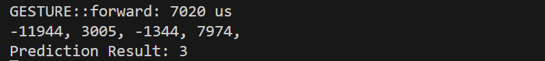
【无softmax层】推理耗时：7020us

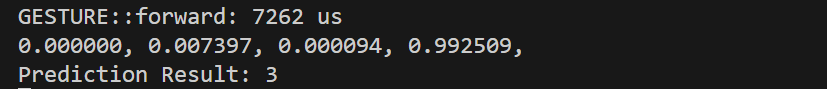
【有softmax层】推理耗时：7262us

参考：
[1]: esp32/esp32-s2 cpu加速建议 🚀
[2]: esp32 cpu时钟设置 240mhz 🚀
[3]: 【esp32-idf】03-1 系统-内存管理 🚀
[4]: esp32 程序的内存模型 🚀

七、应用逻辑设计

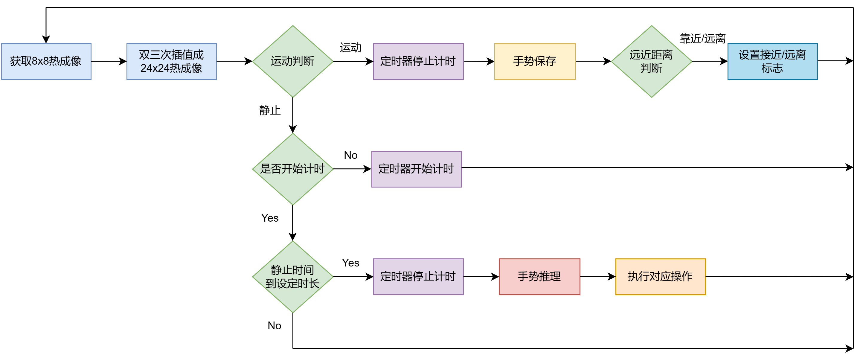
7.1、获取静止状态手势 | 定时器引入

① 获取静止状态手势程序逻辑：

② 定时器引入

对于esp32-s3部署平台，该模型推理过程约7ms，这对于实际应用过程中，能保持较好的实时性，然而，由于该模型未采用rnn/lstm等时序处理模型，所以只能针对某一个动作进行推理。试想一下，当手指由交叉状变成捏住状态，在这个改变过程中的某一个状态，可能被采集被推理为增大，但是实际应该是减小。基于此，通过引入定时器，当某个动作保持一定时间后，才对这个动作进行推理。

esp_timer 内部使用 52 位硬件定时器，对于 esp32-s3 使用的是 systimer。其 api 集支持单次定时器和周期定时器、微秒级的时间分辨率。

定时器回调可通过以下两种方式调度：

• esp_timer_task：定时器回调函数是从高优先级的 esp_timer 任务中调度的，如果有优先级高于 esp_timer 的其他任务正在运行，则回调调度将延迟，直至 esp_timer 能够运行。
• esp_timer_isr：定时器回调由定时器中断处理程序直接调度。对旨在降低延迟的简单回调，建议使用此途径。

定时器可以以单次模式和周期模式启动。

• 单次模式：定时器计时结束，调用回调函数，随后停止；
• 周期模式：定时器计时结束，调用回调函数，随后重新开始，周而复始。

这里采用单次模式+esp_timer_task配置，api接口如下：

• esp_timer_create：创建定时器；
• esp_timer_delete：删除定时器；
• esp_timer_start_once：启动单次模式定时器；
• esp_timer_stop：停止定时器，下一次启动使用esp_timer_start_once；
• esp_timer_get_time：获取从boot开始时间，单位为微秒。

多任务中存在对临界资源的访问，这里通过【互斥锁】加以保护。

测试代码：

#include "esp_timer.h"

esp_timer_handle_t oneshot_timer;
volatile char stillness_time_flag = 0; // 临界资源
semaphorehandle_t xsemaphore = null;
static const char* tag = "example";

static void oneshot_timer_callback(void* arg)
{
    xsemaphoretake(xsemaphore, portmax_delay);
    stillness_time_flag = 1;
    xsemaphoregive(xsemaphore);
}

const esp_timer_create_args_t oneshot_timer_args = {
            .callback = &oneshot_timer_callback,
            /* argument specified here will be passed to timer callback function */
            .arg = null,
            .name = "one-shot"};

extern "c" void app_main(void)
{
	esp_error_check(esp_timer_create(&oneshot_timer_args, &oneshot_timer)); //定时器
    xsemaphore = xsemaphorecreatemutex(); //创建互斥量
    assert(xsemaphore != null);
	esp_logi(tag, "time since boot: %lld us", esp_timer_get_time());
	esp_timer_stop(oneshot_timer);
	usleep(2000000); 休眠2s
	esp_timer_start_once(oneshot_timer, 200000);
    esp_logi(tag, "time since boot: %lld us", esp_timer_get_time());
}

参考：
[1]: 高分辨率定时器（esp 定时器） 🚀
[2]: esp_timer_example_main.c 🚀

---

7.2、交互方式选择：交互方式1

到这一步，通过上述动作设定，只需要最后静止的动作是训练的那些动作，就能完成捏住/增加/减小/松开的操作。

• 捏住状态： 选中操作对象；
• 捏住+上移：向右移动，选择操作对象；
• 捏住+下移：向左移动，选择操作对象；
• 交叉状态：操作对象增加；
• 松开状态：操作对象减小；
• 背景状态：取消对象选中。

7.3、交互方式选择：交互方式2

• 捏住=>交叉：操作对象增加；【判断逻辑同交互方式1】
• 交叉=>捏住：操作对象减小；
• 捏住=>松开：操作对象取消选择；【只需要判断最后一个动作即可】
• 松开=>捏住：选中操作对象；
• 捏住+上移：向右移动，选择操作对象；【判断逻辑同交互方式1】
• 捏住+下移：向左移动，选择操作对象。【判断逻辑同交互方式1】

对于交互方式2，在运动过程中，边采集数据边推理，一些动作未加入训练集中训练，所以存在推理错误的情况，然而该组动作最后的操作结果依据这些操作序列得出，就可能导致判断出错。所所所所所以，上面的逻辑是理想的推理！

交互方式切换使用条件编译的方式进行选择：gesture_display.h文件下

#define interactive_methods 1 // 1表示交互方式1, 2表示交互方式2

八、others

8.1、跑一下示例程序（mnist）

1. 下载 esp-dl，可以使用以下命令，当然也可以直接在 github 🚀网页中下载；

git clone https://github.com/espressif/esp-dl.git

2. 打开终端 esp-idf 5.0 cmd，进入 tutorial/convert_tool_example 文件夹：

c: # windows下切换到c盘
dir # 查看当前路径下的文件列表
cd ~/esp-dl/tutorial/convert_tool_example # 切换路径

3. 使用以下命令设置目标芯片：（当前芯片为 esp32s3）

idf.py set-target esp32s3

4. 将psram模式设置为 octal mode psram：终端输入idf.py menuconfig => component config => esp psram => spi ram config => moda (quad/oct) of spi ram chip in use (quad mode psram) => octal mode psram

5. 烧录固件，打印结果

idf.py flash monitor

参考：获取 esp-dl 并运行示例 🚀

8.2、数据集补充程序

对于分类任务，或多或少有些类别没有被添加到数据集，且当前网络无法做到正确推理，所以在前面的基础上写了个数据集补充程序。

程序分为：pc端上位机（python）和 esp32端下位机（c/c++）

程序操作步骤：

1. 运行上位机程序，马上重启esp32；
2. esp32采集手势数据（只要一直在运动就不停止数据采集，当停止采集后，就开始推理，并将推理结果发送到上位机）；
3. 上位机中输入label(0-背景/1-增加/2-捏住/3-减小)或者放弃(4-不添加该数据)；
4. 下位机收到数字后，若为标签数值，则将手势数据上传，若为放弃，则丢弃数据；
5. 然后，开始新一轮的循环。