在日常开发中,我们经常会遇到 sql 执行缓慢的问题。此时,mysql explain 便是排查性能瓶颈的“利器”——它能清晰展示 sql 的执行计划,帮助我们判断索引是否生效、是否存在全表扫描、是否需要优化排序等。本文将从测试环境搭建开始,逐步拆解 explain 的核心字段含义,并通过实战案例讲解如何利用它优化 sql 性能,最后介绍 mysql 8.0 带来的执行计划新特性。
一、准备:搭建测试环境
为了让大家更直观地理解 explain 的用法,我们先创建一套测试数据。以下 sql 可直接在 mysql 中执行,用于生成数据库、表结构及模拟数据。
1.1 创建数据库与表
-- 1. 创建测试数据库 martin
create database martin;
use martin;
-- 2. 创建表 t1(含主键与普通索引)
drop table if exists t1;
create table `t1` (
  `id` int not null auto_increment,
  `a` int default null,
  `b` int default null,
  `create_time` datetime not null default current_timestamp comment '记录创建时间',
  `update_time` datetime not null default current_timestamp on update current_timestamp comment '记录更新时间',
  primary key (`id`),  -- 主键索引
  key `idx_a` (`a`),   -- 普通索引 a
  key `idx_b` (`b`)    -- 普通索引 b
) engine=innodb default charset=utf8mb4;
-- 3. 创建存储过程,批量插入 1000 条数据
drop procedure if exists insert_t1;
delimiter ;;
create procedure insert_t1()
begin
  declare i int;
  set i = 1;
  while (i <= 1000) do
    insert into t1(a, b) values(i, i);
    set i = i + 1;
  end while;
end;;
delimiter ;
call insert_t1();  -- 调用存储过程插入数据
-- 4. 复制 t1 表结构与数据到 t2
drop table if exists t2;
create table t2 like t1;
insert into t2 select * from t1;
1.2 初识 explain
执行以下语句,即可查看 sql 的执行计划:
explain select * from t1 where b = 100;
执行后会返回一张包含 12 个字段的表格,这些字段便是我们分析 sql 性能的核心依据。接下来,我们逐一拆解这些字段的含义。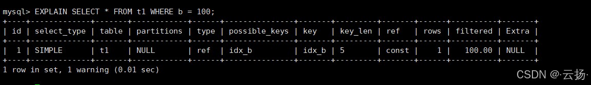
二、explain 核心字段详解
explain 结果包含 id、select_type、table、type 等 12 个字段,其中 select_type、type、key、key_len、extra 是需要重点关注的核心字段(下文已标粗)。
| 列名 | 解释 |
|---|---|
| id | 查询编号,用于标识多表关联或子查询中的执行顺序 |
| select_type | 查询类型,区分简单查询、子查询、联合查询等 |
| table | 执行查询涉及的表 |
| partitions | 匹配的分区(仅分区表有效,非分区表为 null) |
| type | 表连接/查询类型,直接反映查询性能(从优到差排序) |
| possible_keys | mysql 认为可能用到的索引(仅供参考,不一定实际使用) |
| key | 实际使用的索引(若为 null,说明未使用索引) |
| key_len | 实际使用的索引长度(可用于判断联合索引的生效列数) |
| ref | 与索引比较的列或常量(如 const 表示与常量比较) |
| rows | 预估需要扫描的行数(innodb 为估值,非精确值) |
| filtered | 按条件筛选后的行百分比(值越高,筛选效果越好) |
| extra | 附加信息,包含性能优化的关键提示(如是否全表扫描、是否使用临时表等) |
2.1 select_type:区分查询类型
select_type 用于标识查询的复杂程度,常见值如下:
| select_type 值 | 解释 |
|---|---|
| simple | 简单查询(无关联、无子查询),最常见的类型 |
| primary | 复杂查询中的最外层查询(如子查询的外层、联合查询的第一个查询) |
| union | 联合查询中第二个及以后的查询(如 a union b 中的 b) |
| dependent union | 依赖外部查询结果的联合查询(外层查询的结果影响内层联合查询) |
| subquery | 子查询中的第一个查询(不依赖外层结果) |
| dependent subquery | 依赖外层查询结果的子查询(外层每行都需触发子查询执行) |
| derived | 派生表查询(如 from 子句中的子查询,mysql 会先将结果存入临时表) |
| materialized | 物化子查询(mysql 将子查询结果缓存为临时表,避免重复执行) |
示例:子查询的 select_type
explain select * from t1 where a = (select a from t2 where id = 10);
此时,子查询 (select a from t2 where id = 10) 的 select_type 为 subquery,外层查询的 select_type 为 primary。
2.2 type:判断查询性能等级
type 是 explain 中最核心的字段之一,它表示表的查询/连接方式,性能从优到差依次为:system > const > eq_ref > ref > fulltext > ref_or_null > index_merge > unique_subquery > index_subquery > range > index > all
| type 值 | 解释 | 适用场景示例 |
|---|---|---|
| system | 表仅有 1 行数据(仅 myisam/memory 引擎支持),性能最优 | 查询 myisam 引擎的单行情报表 |
| const | 基于主键/唯一索引的等值查询,仅返回 1 行结果 | select * from t1 where id = 100 |
| eq_ref | 多表关联时,基于主键/唯一索引的等值匹配(每行仅匹配 1 行) | select * from t1 join t2 on t1.id = t2.id |
| ref | 基于普通索引的等值查询,可能返回多行 | select * from t1 where b = 100(b 有普通索引) |
| range | 基于索引的范围查询(如 >、<、between、in) | select * from t1 where a between 100 and 200 |
| index | 全索引扫描(比全表扫描快,因索引文件更小) | select a from t1(a 有索引,仅扫描索引树) |
| all | 全表扫描(性能最差,需避免) | select * from t1 where create_time = '2024-01-01'(create_time 无索引) |
优化建议:实际开发中,应尽量保证 type 至少达到 range 级别,避免 index 或 all(全表/全索引扫描)。
2.3 key_len:判断索引生效长度
key_len 表示实际使用的索引字节数,可用于判断 联合索引的生效列数(需结合字段类型计算)。常见字段类型的 key_len 计算规则如下:
| 列类型 | key_len 计算方式 | 备注 |
|---|---|---|
| int(允许 null) | 4 + 1 = 5 字节 | int 占 4 字节,null 需 1 字节标记 |
| int(not null) | 4 字节 | 无 null 标记,仅字段本身长度 |
| bigint(允许 null) | 8 + 1 = 9 字节 | bigint 占 8 字节 |
| char(30) utf8(null) | 30 * 3 + 1 = 91 字节 | utf8 中 1 字符占 3 字节,char 是定长类型 |
| varchar(30) utf8(null) | 30 * 3 + 2 + 1 = 93 字节 | varchar 是变长类型,需 2 字节存储长度,null 需 1 字节标记 |
| datetime(mysql 8.0) | 5 + 1 = 6 字节 | 5.6.4 后 datetime 优化为 5 字节存储,null 需 1 字节 |
示例:联合索引 idx_a_b(a, b),若查询 where a = 100,key_len 为 5(int 允许 null);若查询 where a = 100 and b = 200,key_len 为 5 + 5 = 10 字节,说明联合索引的两列均生效。
2.4 extra:性能优化的关键提示
extra 字段包含大量优化相关的细节,常见值及优化建议如下:
| extra 值 | 解释 | 优化建议 |
|---|---|---|
| using filesort | 非索引排序(需在内存/磁盘排序,性能差) | 给排序字段添加索引(如 order by create_time 需 idx_create_time) |
| using temporary | 创建临时表存储中间结果(常见于无索引的 group by) | 给 group by 字段添加索引 |
| using index | 覆盖索引(仅扫描索引即可获取结果,无需回表,性能优) | 保持查询字段在索引中(如 select a from t1 用 idx_a) |
| using where | 需通过 where 筛选结果(若结合全表扫描,需优化) | 给 where 条件字段添加索引 |
| impossible where | where 条件恒为 false(如 1 < 0),无数据返回 | 检查条件逻辑,避免无效查询 |
| using join buffer | 关联查询中,被驱动表无索引,需用连接缓冲区(性能差) | 给被驱动表的关联字段添加索引 |
| select tables optimized away | 用聚合函数(max/min)访问索引字段,mysql 直接优化为索引查找 | 无需优化,已是最优状态 |
示例:using filesort 优化前:
-- 无索引的 order by,出现 using filesort
explain select * from t1 order by create_time;
优化后(添加索引):
alter table t1 add index idx_create_time(create_time);
explain select * from t1 order by create_time;  -- 无 using filesort
三、实战:explain 优化案例
理论结合实践才能更好地掌握 explain,以下通过 3 个实战案例,展示如何用 explain 定位并解决性能问题。
3.1 案例 1:对比有无索引的执行计划
索引是优化 sql 的核心手段,我们通过 explain 对比“主键查询”“有索引查询”“无索引查询”的差异:
| 查询场景 | sql 语句 | type 类型 | key 索引 | 性能结论 |
|---|---|---|---|---|
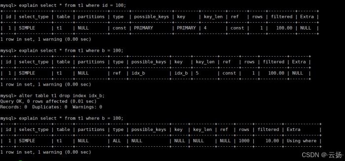
| 主键查询(有唯一索引) | explain select * from t1 where id = 100 | const | primary | 最优,仅扫描 1 行 |
| 普通索引查询 | explain select * from t1 where b = 100 | ref | idx_b | 优秀,扫描少量行 |
| 无索引查询(删除 idx_b) | alter table t1 drop index idx_b;explain select * from t1 where b = 100 | all | null | 最差,全表扫描 1000 行 |
结论:索引能显著降低扫描行数,将 type 从 all(全表)提升至 ref 或 const。
3.2 案例 2:分析分区表的执行计划
对于海量数据,分区表是常用方案。explain 的 partitions 字段可展示查询命中的分区,帮助验证分区有效性。
步骤 1:创建分区表
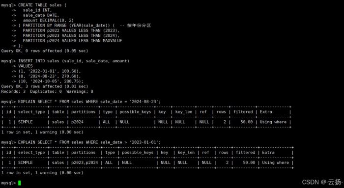
create table sales (
  sale_id int,
  sale_date date,
  amount decimal(10, 2)
) partition by range (year(sale_date)) (  -- 按年份分区
  partition p2022 values less than (2023),
  partition p2023 values less than (2024),
  partition p2024 values less than maxvalue
);
-- 插入 2022-2024 年数据
insert into sales (sale_id, sale_date, amount)
values
(1, '2022-01-01', 100.50),
(8, '2024-08-23', 270.60),
(10, '2024-10-05', 280.75);
步骤 2:查看分区执行计划
-- 查询 2024 年数据,仅命中 p2024 分区
explain select * from sales where sale_date = '2024-08-23';
-- 查询 2023 年后数据,命中 p2023、p2024 分区
explain select * from sales where sale_date > '2023-01-01';
此时 partitions 字段会显示 p2024 或 p2023,p2024,说明分区生效,避免了全分区扫描。
3.3 案例 3:排查正在执行的慢查询
当生产环境出现慢查询时,可通过 explain for connection 查看其执行计划,无需等待查询结束。
步骤 1:构造慢查询
在窗口 1 执行一条含 sleep(100) 的慢查询:
select *, sleep(100) from t1 limit 1; -- 执行时间约 100 秒

步骤 2:获取连接 id
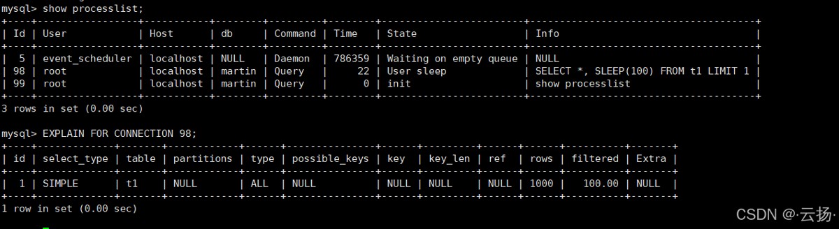
在窗口 2 执行 show processlist,找到慢查询的 id(如 12):
show processlist;
步骤 3:查看慢查询执行计划
explain for connection 12; -- 12 为慢查询的 id
通过此方式,可快速定位慢查询是否存在全表扫描、未使用索引等问题,及时优化。
四、mysql 8.0 执行计划新特性
mysql 8.0 对 explain 进行了增强,新增了 树状执行计划 和 explain analyze,进一步提升了优化效率。
4.1 树状执行计划(format=tree)
从 mysql 8.0.16 开始,支持输出树状结构的执行计划,更直观地展示查询逻辑(如关联顺序、过滤条件)。
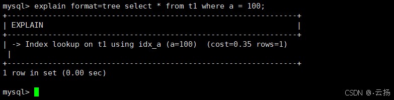
explain format=tree select * from t1 where a = 100;
执行结果如下(结构清晰,包含预估成本和行数):
-> rows fetched before execution (cost=0.25 rows=1)
    -> index lookup on t1 using idx_a (a=100) (cost=0.25 rows=1)
4.2 explain analyze(实际执行分析)
从 mysql 8.0.18 开始,explain analyze 会实际执行 sql,并返回更精确的执行信息(如实际扫描行数、执行时间、循环次数),解决了传统 explain 估值不准的问题。
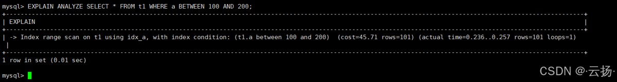
explain analyze select * from t1 where a between 100 and 200;
执行结果包含以下关键信息:
actual time: 实际执行时间(如0.02秒)actual rows: 实际扫描行数(如101行)loops: 循环次数(如1次)
注意:explain analyze 会执行 sql,若为写操作(如 insert/update),需先备份数据或在测试环境使用。
五、总结
explain 是 mysql 性能优化的“基石”,掌握它的核心要点可帮助我们快速定位问题:
- 重点关注字段:
type(性能等级)、key(实际索引)、extra(优化提示); - 索引优化原则:避免
type=all(全表扫描),消除using filesort和using temporary; - 实战技巧:用
explain for connection排查慢查询,用 mysql 8.0 的explain analyze获取精确执行信息。
希望本文能帮助你更好地利用 explain 优化 sql 性能,让数据库查询更高效!
到此这篇关于mysql explain 从入门到实战完全指南的文章就介绍到这了,更多相关mysql explain实战内容请搜索代码网以前的文章或继续浏览下面的相关文章希望大家以后多多支持代码网!


发表评论