【动手学深度学习】深入浅出深度学习之线性神经网络_神经网络

%matplotlib inline
import math
import time
import numpy as np
import torch
from d2l import torch as d2l

n = 10000
a = torch.ones([n])
b = torch.ones([n])

class timer:  #@save
    """记录多次运行时间"""
    def __init__(self):
        self.times = []
        self.start()

    def start(self):
        """启动计时器"""
        self.tik = time.time()

    def stop(self):
        """停止计时器并将时间记录在列表中"""
        self.times.append(time.time() - self.tik)
        return self.times[-1]

    def avg(self):
        """返回平均时间"""
        return sum(self.times) / len(self.times)

    def sum(self):
        """返回时间总和"""
        return sum(self.times)

    def cumsum(self):
        """返回累计时间"""
        return np.array(self.times).cumsum().tolist()

c = torch.zeros(n)
timer = timer()
for i in range(n):
    c[i] = a[i] + b[i]
f'{timer.stop():.5f} sec'

输出结果

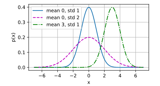
🌻1.2 正态分布与平方损失

def normal(x, mu, sigma):
    p = 1 / math.sqrt(2 * math.pi * sigma**2)
    return p * np.exp(-0.5 / sigma**2 * (x - mu)**2)

# 再次使用numpy进行可视化
x = np.arange(-7, 7, 0.01)

# 均值和标准差对
params = [(0, 1), (0, 2), (3, 1)]
d2l.plot(x, [normal(x, mu, sigma) for mu, sigma in params], xlabel='x',
         ylabel='p(x)', figsize=(4.5, 2.5),
         legend=[f'mean {mu}, std {sigma}' for mu, sigma in params])

输出结果

🌼2. 线性回归的从零开始实现

%matplotlib inline
import random
import torch
from d2l import torch as d2l

🌻2.1. 生成数据集

def synthetic_data(w, b, num_examples):  #@save
    """生成y=xw+b+噪声"""
    x = torch.normal(0, 1, (num_examples, len(w)))
    y = torch.matmul(x, w) + b
    y += torch.normal(0, 0.01, y.shape)
    return x, y.reshape((-1, 1))

true_w = torch.tensor([2, -3.4])
true_b = 4.2
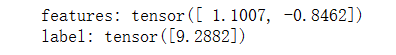
features, labels = synthetic_data(true_w, true_b, 1000)

print('features:', features[0],'\nlabel:', labels[0])

输出结果

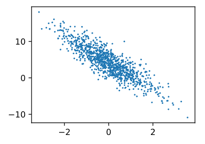
d2l.set_figsize()
d2l.plt.scatter(features[:, 1].detach().numpy(), labels.detach().numpy(), 1);

输出结果

🌻2.2 读取数据集

def data_iter(batch_size, features, labels):
    num_examples = len(features)
    indices = list(range(num_examples))
    # 这些样本是随机读取的，没有特定的顺序
    random.shuffle(indices)
    for i in range(0, num_examples, batch_size):
        batch_indices = torch.tensor(
            indices[i: min(i + batch_size, num_examples)])
        yield features[batch_indices], labels[batch_indices]

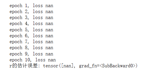
batch_size = 10

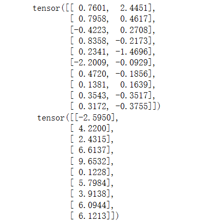
for x, y in data_iter(batch_size, features, labels):
    print(x, '\n', y)
    break

输出结果

🌻2.3. 初始化模型参数

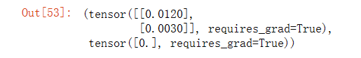
w = torch.normal(0, 0.01, size=(2,1), requires_grad=true)
b = torch.zeros(1, requires_grad=true)
w,b

输出结果

🌻2.4. 定义模型

def linreg(x, w, b):  #@save
    """线性回归模型"""
    return torch.matmul(x, w) + b

🌻2.5. 定义损失函数

def squared_loss(y_hat, y):  #@save
    """均方损失"""
    return (y_hat - y.reshape(y_hat.shape)) ** 2 / 2

🌻2.6. 定义优化算法

def sgd(params, lr, batch_size):  #@save
    """小批量随机梯度下降"""
    with torch.no_grad():
        for param in params:
            param -= lr * param.grad / batch_size
            param.grad.zero_()

🌻2.7. 训练

lr = 0.03
num_epochs = 3
net = linreg
loss = squared_loss

for epoch in range(num_epochs):
    for x, y in data_iter(batch_size, features, labels):
        l = loss(net(x, w, b), y)  # x和y的小批量损失
        # 因为l形状是(batch_size,1)，而不是一个标量。l中的所有元素被加到一起，
        # 并以此计算关于[w,b]的梯度
        l.sum().backward()
        sgd([w, b], lr, batch_size)  # 使用参数的梯度更新参数
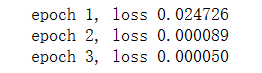
    with torch.no_grad():
        train_l = loss(net(features, w, b), labels)
        print(f'epoch {epoch + 1}, loss {float(train_l.mean()):f}')

输出结果

print(f'w的估计误差: {true_w - w.reshape(true_w.shape)}')
print(f'b的估计误差: {true_b - b}')

输出结果

🌻2.8 小结

🌻2.9 练习

1.如果我们将权重初始化为零，会发生什么。算法仍然有效吗？

# 在单层网络中(一层线性回归层)，将权重初始化为零时可以的，但是网络层数加深后，在全连接的情况下，
# 在反向传播的时候，由于权重的对称性会导致出现隐藏神经元的对称性，使得多个隐藏神经元的作用就如同
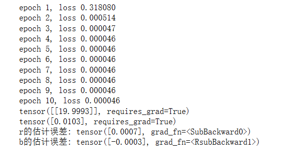
# 1个神经元，算法还是有效的，但是效果不大好。参考：https://zhuanlan.zhihu.com/p/75879624。

2.假设试图为电压和电流的关系建立一个模型。自动微分可以用来学习模型的参数吗？

# 可以的，建立模型u=iw+b，然后采集(u，i)的数据集，通过自动微分即可学习w和b的参数。
import torch
import random
from d2l import torch as d2l
#生成数据集
def synthetic_data(r, b, num_examples):
    i = torch.normal(0, 1, (num_examples, len(r)))
    u = torch.matmul(i, r) + b
    u += torch.normal(0, 0.01, u.shape) # 噪声
    return i, u.reshape((-1, 1)) # 标量转换为向量

true_r = torch.tensor([20.0])
true_b = 0.01
features, labels = synthetic_data(true_r, true_b, 1000)

#读取数据集
def data_iter(batch_size, features, labels):
    num_examples = len(features)
    indices = list(range(num_examples))
    random.shuffle(indices)
    for i in range(0, num_examples, batch_size):
        batch_indices = torch.tensor(indices[i: min(i + batch_size, num_examples)])
        yield features[batch_indices],labels[batch_indices]
        
batch_size = 10
# 初始化权重
r = torch.normal(0,0.01,size = ((1,1)), requires_grad = true)
b = torch.zeros(1, requires_grad = true)

# 定义模型
def linreg(i, r, b):
    return torch.matmul(i, r) + b
# 损失函数
def square_loss(u_hat, u):
    return (u_hat - u.reshape(u_hat.shape)) ** 2/2
# 优化算法
def sgd(params, lr, batch_size):
    with torch.no_grad():
        for param in params:
            param -= lr * param.grad/batch_size
            param.grad.zero_()

lr = 0.03
num_epochs = 10
net = linreg
loss = square_loss

for epoch in range(num_epochs):
    for i, u in data_iter(batch_size, features, labels):
        l = loss(net(i, r, b), u)
        l.sum().backward()
        sgd([r, b], lr, batch_size)
    with torch.no_grad():
        train_l = loss(net(features, r, b), labels)
        print(f'epoch {epoch + 1}, loss {float(train_l.mean()):f}')
print(r)
print(b)
print(f'r的估计误差: {true_r - r.reshape(true_r.shape)}')
print(f'b的估计误差: {true_b - b}')

输出结果

3.能基于普朗克定律使用光谱能量密度来确定物体的温度吗？

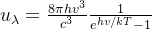
$u _ { \lambda } = \frac { 8 \pi h v ^ { 3 } } { c ^ { 3 } } \frac { 1 } { e ^ { h v / k t } - 1 }$

# 3
# 普朗克公式
# x:波长
# t:温度
import torch
import random
from d2l import torch as d2l


#生成数据集
def synthetic_data(x, num_examples):
    t = torch.normal(0, 1, (num_examples, len(x)))
    u = c1 / ((x ** 5) * ((torch.exp(c2 / (x * t))) - 1));
    u += torch.normal(0, 0.01, u.shape) # 噪声
    return t, u.reshape((-1, 1)) # 标量转换为向量


c1 = 3.7414*10**8  # c1常量
c2 = 1.43879*10**4  # c2常量
true_x = torch.tensor([500.0])

features, labels = synthetic_data(true_x, 1000)


#读取数据集
def data_iter(batch_size, features, labels):
    num_examples = len(features)
    indices = list(range(num_examples))
    random.shuffle(indices)
    for i in range(0, num_examples, batch_size):
        batch_indices = torch.tensor(indices[i: min(i + batch_size, num_examples)])
        yield features[batch_indices],labels[batch_indices]

batch_size = 10
# 初始化权重
x = torch.normal(0,0.01,size = ((1,1)), requires_grad = true)


# 定义模型
def planck_formula(t, x):
    return c1 / ((x ** 5) * ((torch.exp(c2 / (x * t))) - 1))
# 损失函数
def square_loss(u_hat, u):
    return (u_hat - u.reshape(u_hat.shape)) ** 2/2
# 优化算法
def sgd(params, lr, batch_size):
    with torch.no_grad():
        for param in params:
            param -= lr * param.grad/batch_size
            param.grad.zero_()

lr = 0.001
num_epochs = 10
net = planck_formula
loss = square_loss

for epoch in range(num_epochs):
    for t, u in data_iter(batch_size, features, labels):
        l = loss(net(t, x), u)
        l.sum().backward()
        sgd([x], lr, batch_size)
    with torch.no_grad():
        train_l = loss(net(features, x), labels)
        print(f'epoch {epoch + 1}, loss {float(train_l.mean()):f}')

print(f'r的估计误差: {true_x - x.reshape(true_x.shape)}')

输出结果

4.计算二阶导数时可能会遇到什么问题？这些问题可以如何解决？

#  一阶导数的正向计算图无法直接获得，可以通过保存一阶导数的计算图使得可以求二阶导数(create_graph和retain_graph都置为true，
# 保存原函数和一阶导数的正向计算图)。实验如下：
import torch

x = torch.randn((2), requires_grad=true)
y = x**3

dy = torch.autograd.grad(y, x, grad_outputs=torch.ones(x.shape),
                         retain_graph=true, create_graph=true)
dy2 = torch.autograd.grad(dy, x, grad_outputs=torch.ones(x.shape))

dy_ = 3*x**2
dy2_ = 6*x

print("======================================================")
print(dy, dy_)
print("======================================================")
print(dy2, dy2_)

输出结果

5.为什么在squared_loss函数中需要使用reshape函数？

# 以防y^和y，一个是行向量、一个是列向量，使用reshape，可以确保shape一样。

6.尝试使用不同的学习率，观察损失函数值下降的快慢。

# ①学习率过大前期下降很快，但是后面不容易收敛；
# ②学习率过小损失函数下降会很慢。

7.如果样本个数不能被批量大小整除，data_iter函数的行为会有什么变化？

# 报错。

🌼3. 线性回归的简洁实现

（1）使用jupyter notebook新增的pytorch环境新建ipynb文件，完成线性回归的简洁实现的实验代码与练习结果如下：

🌻3.1. 生成数据集

import numpy as np
import torch
from torch.utils import data
from d2l import torch as d2l

true_w = torch.tensor([2, -3.4])
true_b = 4.2
features, labels = d2l.synthetic_data(true_w, true_b, 1000)

🌻3.2. 读取数据集

def load_array(data_arrays, batch_size, is_train=true):  #@save
    """构造一个pytorch数据迭代器"""
    dataset = data.tensordataset(*data_arrays)
    return data.dataloader(dataset, batch_size, shuffle=is_train)

batch_size = 10
data_iter = load_array((features, labels), batch_size)

next(iter(data_iter))

输出结果

🌻3.3 定义模型

# nn是神经网络的缩写
from torch import nn

net = nn.sequential(nn.linear(2, 1))

🌻3.4 初始化模型参数

net[0].weight.data.normal_(0, 0.01)
net[0].bias.data.fill_(0)

输出结果

🌻3.5 定义损失函数

loss = nn.mseloss()

🌻3.6 定义优化算法

trainer = torch.optim.sgd(net.parameters(), lr=0.03)

🌻3.7 训练

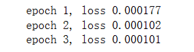
num_epochs = 3
for epoch in range(num_epochs):
    for x, y in data_iter:
        l = loss(net(x) ,y)
        trainer.zero_grad()
        l.backward()
        trainer.step()
    l = loss(net(features), labels)
    print(f'epoch {epoch + 1}, loss {l:f}')

输出结果

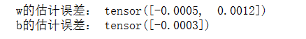
w = net[0].weight.data
print('w的估计误差：', true_w - w.reshape(true_w.shape))
b = net[0].bias.data
print('b的估计误差：', true_b - b)

输出结果

🌻3.8 小结

我们可以使用pytorch的高级api更简洁地实现模型。
在pytorch中，data模块提供了数据处理工具，nn模块定义了大量的神经网络层和常见损失函数。
我们可以通过_结尾的方法将参数替换，从而初始化参数。

🌻3.9 练习

1.如果将小批量的总损失替换为小批量损失的平均值，需要如何更改学习率？

# 将学习率除以batchsize。

2.查看深度学习框架文档，它们提供了哪些损失函数和初始化方法？

用huber损失代替原损失，即

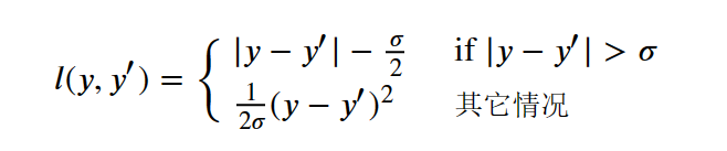
# huber损失可以用torch自带的函数解决
torch.nn.smoothl1loss()
# 也可以自己写
import torch.nn as nn
import torch.nn.functional as f

class huberloss(nn.module):
    def __init__(self, sigma):
        super(huberloss, self).__init__()
        self.sigma = sigma
    def forward(self, y, y_hat):
        if f.l1_loss(y, y_hat) > self.sigma:
            loss = f.l1_loss(y, y_hat) - self.sigma/2
        else:
            loss = (1/(2*self.sigma))*f.mse_loss(y, y_hat)
        
        return loss

#%%
import numpy as np
import torch
from torch.utils import data
from d2l import torch as d2l

#%%
true_w = torch.tensor([2, -3.4])
true_b = 4.2
features, labels = d2l.synthetic_data(true_w, true_b, 1000)

def load_array(data_arrays, batch_size, is_train = true): #@save
    '''pytorch数据迭代器'''
    dataset = data.tensordataset(*data_arrays) # 把输入的两类数据一一对应；*表示对list解开入参
    return data.dataloader(dataset, batch_size, shuffle = is_train) # 重新排序

batch_size = 10
data_iter = load_array((features, labels), batch_size) # 和手动实现中data_iter使用方法相同

#%%
# 构造迭代器并验证data_iter的效果
next(iter(data_iter))  # 获得第一个batch的数据

#%% 定义模型
from torch import nn
net = nn.sequential(nn.linear(2, 1))  # linear中两个参数一个表示输入形状一个表示输出形状
# sequential相当于一个存放各层数据的list，单层时也可以只用linear

#%% 初始化模型参数
# 使用net[0]选择神经网络中的第一层
net[0].weight.data.normal_(0, 0.01) # 正态分布
net[0].bias.data.fill_(0)

#%% 定义损失函数
loss = torch.nn.huberloss()
#%% 定义优化算法
trainer = torch.optim.sgd(net.parameters(), lr=0.03) # optim module中的sgd
#%% 训练
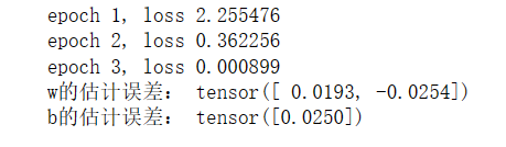
num_epochs = 3
for epoch in range(num_epochs):
    for x, y in data_iter:
        l = loss(net(x), y)
        trainer.zero_grad()
        l.backward()
        trainer.step()
    l = loss(net(features), labels)
    print(f'epoch {epoch+1}, loss {l:f}')

#%% 查看误差
w = net[0].weight.data
print('w的估计误差：', true_w - w.reshape(true_w.shape))
b = net[0].bias.data
print('b的估计误差：', true_b - b)

输出结果

3.如何访问线性回归的梯度？

#假如是多层网络，可以用一个self.xxx=某层，然后在外面通过net.xxx.weight.grad和net.xxx.bias.grad把梯度给拿出来。
net[0].weight.grad
net[0].bias.grad

输出结果

🌞四、实验心得

通过此次实验，我熟悉了pytorch框架以及pytorch的基本概念、数据结构和核心函数；创建了线性回归模型，使用pytorch构建一个简单的线性回归模型；完成了线性回归从零开始实现及其简洁实现以及章节后习题。明白了以下几点：

【动手学深度学习】深入浅出深度学习之线性神经网络

2024年08月02日 • 神经网络 •我要评论

🌞一、实验目的

🌞二、实验准备

🌞三、实验内容

🌼1. 线性回归

🌻1.1 矢量化加速

🌻1.2 正态分布与平方损失

🌼2. 线性回归的从零开始实现

🌻2.1. 生成数据集

🌻2.2 读取数据集

🌻2.3. 初始化模型参数

🌻2.4. 定义模型

🌻2.5. 定义损失函数

🌻2.6. 定义优化算法

🌻2.7. 训练

🌻2.8 小结

🌻2.9 练习

🌼3. 线性回归的简洁实现

🌻3.1. 生成数据集

🌻3.2. 读取数据集

🌻3.3 定义模型

🌻3.4 初始化模型参数

🌻3.5 定义损失函数

🌻3.6 定义优化算法

🌻3.7 训练

🌻3.8 小结

🌻3.9 练习

🌞四、实验心得

相关文章:

论文阅读笔记三遍阅读详解知识图谱入门之作(A Survey on Knowledge Graphs)_知识图谱survey(2)

NLP实战：Pytorch实现6大经典深度学习中文短文本分类-bert+ERNIE+bert_CNN+bert_RNN+bert_RCNN+bert_DPCNN

发表评论


验证码：

【动手学深度学习】深入浅出深度学习之线性神经网络

2024年08月02日 • 神经网络 •我要评论

🌞一、实验目的

🌞二、实验准备

🌞三、实验内容

🌼1. 线性回归

🌻1.1 矢量化加速

🌻1.2 正态分布与平方损失

🌼2. 线性回归的从零开始实现

🌻2.1. 生成数据集

🌻2.2 读取数据集

🌻2.3. 初始化模型参数

🌻2.4. 定义模型

🌻2.5. 定义损失函数

🌻2.6. 定义优化算法

🌻2.7. 训练

🌻2.8 小结

🌻2.9 练习

🌼3. 线性回归的简洁实现

🌻3.1. 生成数据集

🌻3.2. 读取数据集

🌻3.3 定义模型

🌻3.4 初始化模型参数

🌻3.5 定义损失函数

🌻3.6 定义优化算法

🌻3.7 训练

🌻3.8 小结

🌻3.9 练习

🌞四、实验心得

相关文章:

论文阅读笔记 三遍阅读详解知识图谱入门之作(A Survey on Knowledge Graphs)_知识图谱survey(2)

NLP实战：Pytorch实现6大经典深度学习中文短文本分类-bert+ERNIE+bert_CNN+bert_RNN+bert_RCNN+bert_DPCNN

发表评论

论文阅读笔记三遍阅读详解知识图谱入门之作(A Survey on Knowledge Graphs)_知识图谱survey(2)