聚类是什么?
聚类或者聚类分析是无监督学习问题。通常被用作数据分析技术,用来发现大数据中的有趣模型。与监督学习(类似预测模型)不同,聚类算法只解释输入数据,并在特征空间中找到自然组或群集。
一句话概括:聚类技术适用于没有要预测的类,只是将实例划分为自然组的情况
聚类数据集
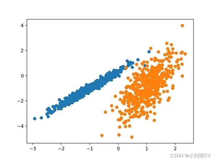
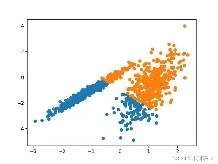
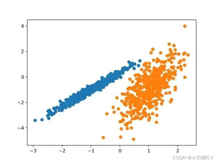
我们将使用 make _ classification ()函数创建一个测试二分类数据集。数据集将有1000个示例,每个类有两个输入要素和一个群集。这些群集在两个维度上是可见的,因此我们可以用散点图绘制数据,并通过指定的群集对图中的点进行颜色绘制。这将有助于了解,至少在测试问题上,群集的识别能力如何。该测试问题中的群集基于多变量高斯,并非所有聚类算法都能有效地识别这些类型的群集。因此,本教程中的结果不应用作比较一般方法的基础。下面列出了创建和汇总合成聚类数据集的示例。
# 综合分类数据集
from numpy import where
from sklearn.datasets import make_classification
from matplotlib import pyplot
# 定义数据集
x, y = make_classification(n_samples=1000, n_features=2, n_informative=2, n_redundant=0, n_clusters_per_class=1, random_state=4)
# 为每个类的样本创建散点图
for class_value in range(2):
# 获取此类的示例的行索引
row_ix = where(y == class_value)
# 创建这些样本的散布
pyplot.scatter(x[row_ix, 0], x[row_ix, 1])
# 绘制散点图
pyplot.show()
聚类算法?
聚类分析的所有目标的核心是被群集的各个对象之间的相似程度(或不同程度)的概念。聚类方法尝试根据提供给对象的相似性定义对对象进行分组。
聚类分析是一个迭代过程,在该过程中,对所识别的群集的主观评估被反馈回算法配置的改变中,直到达到期望或者适当的结果。
scikit-learn库提供了一些主流的聚类算法,下面主要说十种。
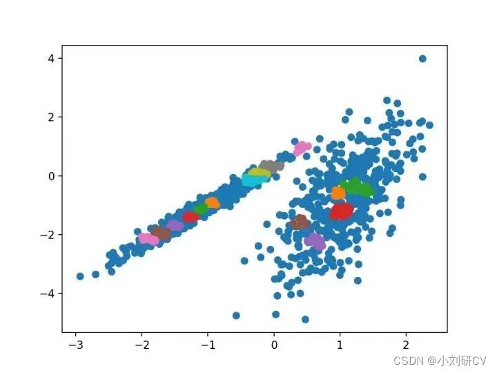
1.亲和力传播
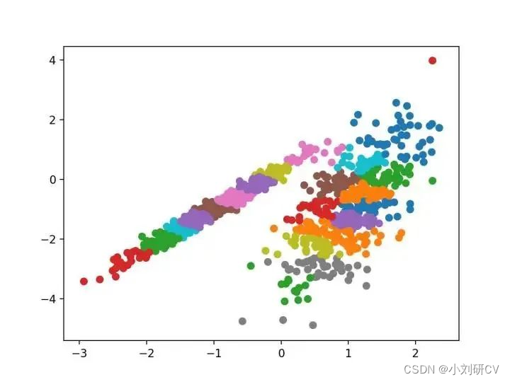
亲和力传播包括找到一组最能概括数据的范例,它作为两对数据点之间相似度的输入度量。在数据点之间交换实值消息,直到一组高质量的范例和相应的群集逐渐出现。
它是通过 affinitypropagation 类实现的,要调整的主要配置是将“ 阻尼 ”设置为0.5到1。
由其指定的群集着色,这种情况下,聚类的效果不好。
亲和力传播代码

# 亲和力传播聚类
from numpy import unique
from numpy import where
from sklearn.datasets import make_classification
from sklearn.cluster import affinitypropagation
from matplotlib import pyplot
# 定义数据集
x, _ = make_classification(n_samples=1000, n_features=2, n_informative=2, n_redundant=0, n_clusters_per_class=1, random_state=4)
# 定义模型
model = affinitypropagation(damping=0.9)
# 匹配模型
model.fit(x)
# 为每个示例分配一个集群
yhat = model.predict(x)
# 检索唯一群集
clusters = unique(yhat)
# 为每个群集的样本创建散点图
for cluster in clusters:
# 获取此群集的示例的行索引
row_ix = where(yhat == cluster)
# 创建这些样本的散布
pyplot.scatter(x[row_ix, 0], x[row_ix, 1])
# 绘制散点图
pyplot.show()
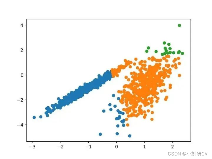
2.聚类聚合
聚类聚合涉及合并实例,直到达到所需群集的数量为止。它是层次聚类方法的更广泛类的一部分,通过agglomerationclustering类实现的,主要配置是“n_clusters”集,是对数据集群集数量的估计。
# 聚合聚类
from numpy import unique
from numpy import where
from sklearn.datasets import make_classification
from sklearn.cluster import agglomerativeclustering
from matplotlib import pyplot
# 定义数据集
x, _ = make_classification(n_samples=1000, n_features=2, n_informative=2, n_redundant=0, n_clusters_per_class=1, random_state=4)
# 定义模型
model = agglomerativeclustering(n_clusters=2)
# 模型拟合与聚类预测
yhat = model.fit_predict(x)
# 检索唯一群集
clusters = unique(yhat)
# 为每个群集的样本创建散点图
for cluster in clusters:
# 获取此群集的示例的行索引
row_ix = where(yhat == cluster)
# 创建这些样本的散布
pyplot.scatter(x[row_ix, 0], x[row_ix, 1])
# 绘制散点图
pyplot.show()

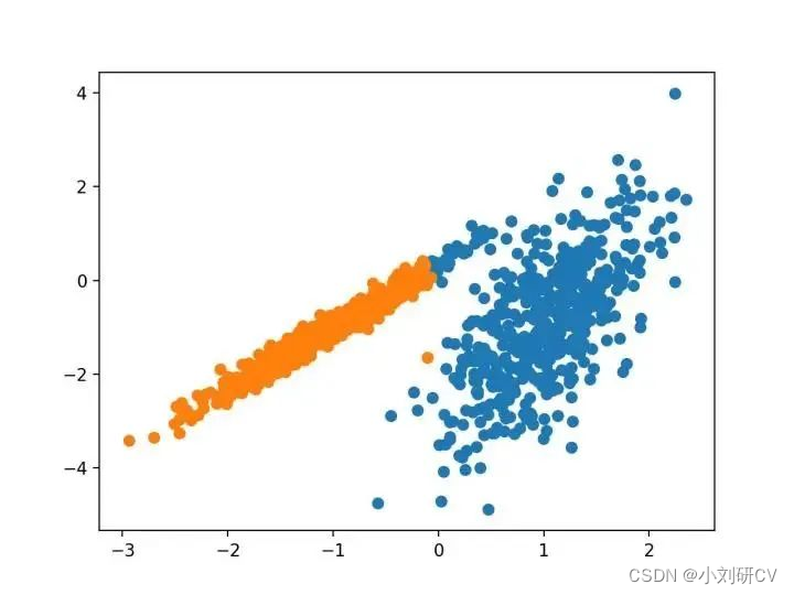
3.birch
birch聚类是平衡迭代减少的缩写,聚类使用层次结构,包括构建一个树状结构,从中提取质心。
它是通过birch类实现的,主要超参数配置是“threshold”和“n_clusters”,后者提供了群集数量的估计。
# birch聚类
from numpy import unique
from numpy import where
from sklearn.datasets import make_classification
from sklearn.cluster import birch
from matplotlib import pyplot
# 定义数据集
x, _ = make_classification(n_samples=1000, n_features=2, n_informative=2, n_redundant=0, n_clusters_per_class=1, random_state=4)
# 定义模型
model = birch(threshold=0.01, n_clusters=2)
# 适配模型
model.fit(x)
# 为每个示例分配一个集群
yhat = model.predict(x)
# 检索唯一群集
clusters = unique(yhat)
# 为每个群集的样本创建散点图
for cluster in clusters:
# 获取此群集的示例的行索引
row_ix = where(yhat == cluster)
# 创建这些样本的散布
pyplot.scatter(x[row_ix, 0], x[row_ix, 1])
# 绘制散点图
pyplot.show()
4.dbscan
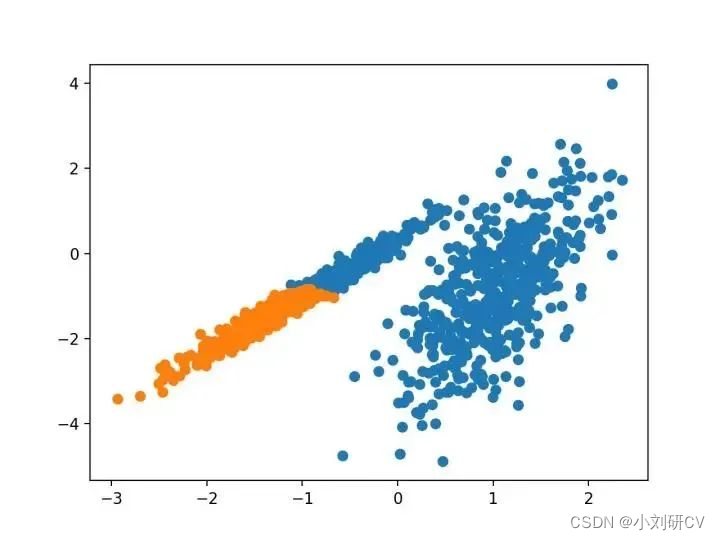
dbscan聚类(其中bdscan是基于密度的空间聚类的噪声应用程序)涉及在域中寻找高密度区域,然后将周围特征空间区域扩展为群集
它是通过dbscan类实现的,主要配置是“eps”和“min_samples”超参数
# dbscan 聚类
from numpy import unique
from numpy import where
from sklearn.datasets import make_classification
from sklearn.cluster import dbscan
from matplotlib import pyplot
# 定义数据集
x, _ = make_classification(n_samples=1000, n_features=2, n_informative=2, n_redundant=0, n_clusters_per_class=1, random_state=4)
# 定义模型
model = dbscan(eps=0.30, min_samples=9)
# 模型拟合与聚类预测
yhat = model.fit_predict(x)
# 检索唯一群集
clusters = unique(yhat)
# 为每个群集的样本创建散点图
for cluster in clusters:
# 获取此群集的示例的行索引
row_ix = where(yhat == cluster)
# 创建这些样本的散布
pyplot.scatter(x[row_ix, 0], x[row_ix, 1])
# 绘制散点图
pyplot.show()
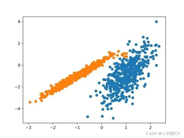
5.k-means
k-均值聚类是最常见的聚类,涉及向群集分配示例,以减少每个群集内的方差。
它将n维种群划分为k个集合,k-均值的过程似乎给出了在类内方差意义上相当有效的分区。
优化的主要超参数为“n_clusters”
# k-means 聚类
from numpy import unique
from numpy import where
from sklearn.datasets import make_classification
from sklearn.cluster import kmeans
from matplotlib import pyplot
# 定义数据集
x, _ = make_classification(n_samples=1000, n_features=2, n_informative=2, n_redundant=0, n_clusters_per_class=1, random_state=4)
# 定义模型
model = kmeans(n_clusters=2)
# 模型拟合
model.fit(x)
# 为每个示例分配一个集群
yhat = model.predict(x)
# 检索唯一群集
clusters = unique(yhat)
# 为每个群集的样本创建散点图
for cluster in clusters:
# 获取此群集的示例的行索引
row_ix = where(yhat == cluster)
# 创建这些样本的散布
pyplot.scatter(x[row_ix, 0], x[row_ix, 1])
# 绘制散点图
pyplot.show()

6.mini-batch k-均值
mini-batch k-均值是 k-均值的修改版本,它使用小批量的样本而不是整个数据集对群集质心进行更新,这可以使大数据集的更新速度更快,并且可能对统计噪声更健壮。
使用 k-均值聚类的迷你批量优化。与经典批处理算法相比,这降低了计算成本的数量级,同时提供了比在线随机梯度下降更好的解决方案。
它是通过 minibatchkmeans 类实现的,要优化的主配置是“ n _ clusters ”超参数,设置为数据中估计的群集数量。下面列出了完整的示例。
# mini-batch k均值聚类
from numpy import unique
from numpy import where
from sklearn.datasets import make_classification
from sklearn.cluster import minibatchkmeans
from matplotlib import pyplot
# 定义数据集
x, _ = make_classification(n_samples=1000, n_features=2, n_informative=2, n_redundant=0, n_clusters_per_class=1, random_state=4)
# 定义模型
model = minibatchkmeans(n_clusters=2)
# 模型拟合
model.fit(x)
# 为每个示例分配一个集群
yhat = model.predict(x)
# 检索唯一群集
clusters = unique(yhat)
# 为每个群集的样本创建散点图
for cluster in clusters:
# 获取此群集的示例的行索引
row_ix = where(yhat == cluster)
# 创建这些样本的散布
pyplot.scatter(x[row_ix, 0], x[row_ix, 1])
# 绘制散点图
pyplot.show()
7.均值漂移聚类
均值漂移聚类涉及到根据特征空间的实例密度来来寻找和调整质心
它是通过 meanshift 类实现的,主要配置是“带宽”超参数。下面列出了完整的示例。
# 均值漂移聚类
from numpy import unique
from numpy import where
from sklearn.datasets import make_classification
from sklearn.cluster import meanshift
from matplotlib import pyplot
# 定义数据集
x, _ = make_classification(n_samples=1000, n_features=2, n_informative=2, n_redundant=0, n_clusters_per_class=1, random_state=4)
# 定义模型
model = meanshift()
# 模型拟合与聚类预测
yhat = model.fit_predict(x)
# 检索唯一群集
clusters = unique(yhat)
# 为每个群集的样本创建散点图
for cluster in clusters:
# 获取此群集的示例的行索引
row_ix = where(yhat == cluster)
# 创建这些样本的散布
pyplot.scatter(x[row_ix, 0], x[row_ix, 1])
# 绘制散点图
pyplot.show()
8.optics
optics聚类是上面dbscan的修改版本。
它不会显式地生成一个数据集的聚类;而是创建表示其基于密度的聚类结构的数据库的增强排序。此群集排序包括相当于密度聚类的信息,该信息对应于范围广泛的参数设置。
它是通过optics类实现的,主要配置是“eps”和“min_samples”超参数。
# optics聚类
from numpy import unique
from numpy import where
from sklearn.datasets import make_classification
from sklearn.cluster import optics
from matplotlib import pyplot
# 定义数据集
x, _ = make_classification(n_samples=1000, n_features=2, n_informative=2, n_redundant=0, n_clusters_per_class=1, random_state=4)
# 定义模型
model = optics(eps=0.8, min_samples=10)
# 模型拟合与聚类预测
yhat = model.fit_predict(x)
# 检索唯一群集
clusters = unique(yhat)
# 为每个群集的样本创建散点图
for cluster in clusters:
# 获取此群集的示例的行索引
row_ix = where(yhat == cluster)
# 创建这些样本的散布
pyplot.scatter(x[row_ix, 0], x[row_ix, 1])
# 绘制散点图
pyplot.show()
9.光谱聚类
光谱聚类是一种通用的聚类算法,取自线性代数
它是通过 spectral 聚类类实现的,而主要的 spectral 聚类是一个由聚类方法组成的通用类,取自线性线性代数。要优化的是“ n _ clusters ”超参数,用于指定数据中的估计群集数量。
# spectral clustering
from numpy import unique
from numpy import where
from sklearn.datasets import make_classification
from sklearn.cluster import spectralclustering
from matplotlib import pyplot
# 定义数据集
x, _ = make_classification(n_samples=1000, n_features=2, n_informative=2, n_redundant=0, n_clusters_per_class=1, random_state=4)
# 定义模型
model = spectralclustering(n_clusters=2)
# 模型拟合与聚类预测
yhat = model.fit_predict(x)
# 检索唯一群集
clusters = unique(yhat)
# 为每个群集的样本创建散点图
for cluster in clusters:
# 获取此群集的示例的行索引
row_ix = where(yhat == cluster)
# 创建这些样本的散布
pyplot.scatter(x[row_ix, 0], x[row_ix, 1])
# 绘制散点图
pyplot.show()
10.高斯混合模型
高斯混合模型总结了一个多变量概率密度函数,顾名思义就是混合了高斯概率分布。它是通过gaussian mixture实现的,
要优化的主要配置是“ n _ clusters ”超参数,用于指定数据中估计的群集数量。
# 高斯混合模型
from numpy import unique
from numpy import where
from sklearn.datasets import make_classification
from sklearn.mixture import gaussianmixture
from matplotlib import pyplot
# 定义数据集
x, _ = make_classification(n_samples=1000, n_features=2, n_informative=2, n_redundant=0, n_clusters_per_class=1, random_state=4)
# 定义模型
model = gaussianmixture(n_components=2)
# 模型拟合
model.fit(x)
# 为每个示例分配一个集群
yhat = model.predict(x)
# 检索唯一群集
clusters = unique(yhat)
# 为每个群集的样本创建散点图
for cluster in clusters:
# 获取此群集的示例的行索引
row_ix = where(yhat == cluster)
# 创建这些样本的散布
pyplot.scatter(x[row_ix, 0], x[row_ix, 1])
# 绘制散点图
pyplot.show()


发表评论