一、线性回归练习
请对数据集(prostate_train.txt 和 prostate_test.txt)使用前四个临床数据(即 lcavol,lweight,lbph,svi)对前列腺特异抗原水平(lpsa)进行预测。所给出的文件中,前 4 列每列代表一个临床数据(即特征),最后一列是测量的前列腺特异抗原水平(即预测目标的真实值);每行代表一个样本。
要求:
- (1) 在不考虑交叉项的情况下,利用 linear regression 对 prostate_train.txt 的数据进行回归,给出回归结果,并对 prostate_test.txt 文件中的患者进行预测,给出结果评价。
- (2) 如果考虑交叉项,是否会有更好的预测结果?请给出你的理由。
import pandas as pd
import numpy as np
import matplotlib.pyplot as plt
from sklearn.linear_model import linearregression
from sklearn.preprocessing import polynomialfeatures # 构建多项式特征,例如交互项
from sklearn.metrics import mean_squared_error, r2_score # 均方误差mse和r方
from sklearn.model_selection import cross_val_score
import seaborn as sns
train_data = pd.read_csv('../data/prostate_train.txt', sep='\t')
test_data = pd.read_csv('../data/prostate_test.txt', sep='\t')
train_data.head()
| lcavol | lweight | lbph | svi | lpsa | |
|---|---|---|---|---|---|
| 0 | -0.579818 | 2.769459 | -1.386294 | 0 | -0.430783 |
| 1 | -0.994252 | 3.319626 | -1.386294 | 0 | -0.162519 |
| 2 | -0.510826 | 2.691243 | -1.386294 | 0 | -0.162519 |
| 3 | -1.203973 | 3.282789 | -1.386294 | 0 | -0.162519 |
| 4 | 0.751416 | 3.432373 | -1.386294 | 0 | 0.371564 |
train_data.describe() # 显然svi这列是0-1变量,其他变量为浮点型数据
| lcavol | lweight | lbph | svi | lpsa | |
|---|---|---|---|---|---|
| count | 67.000000 | 67.000000 | 67.000000 | 67.000000 | 67.000000 |
| mean | 1.313492 | 3.626108 | 0.071440 | 0.223881 | 2.452345 |
| std | 1.242590 | 0.476601 | 1.463655 | 0.419989 | 1.207812 |
| min | -1.347074 | 2.374906 | -1.386294 | 0.000000 | -0.430783 |
| 25% | 0.488279 | 3.330360 | -1.386294 | 0.000000 | 1.667306 |
| 50% | 1.467874 | 3.598681 | -0.051293 | 0.000000 | 2.568788 |
| 75% | 2.349065 | 3.883610 | 1.547506 | 0.000000 | 3.365188 |
| max | 3.821004 | 4.780383 | 2.326302 | 1.000000 | 5.477509 |
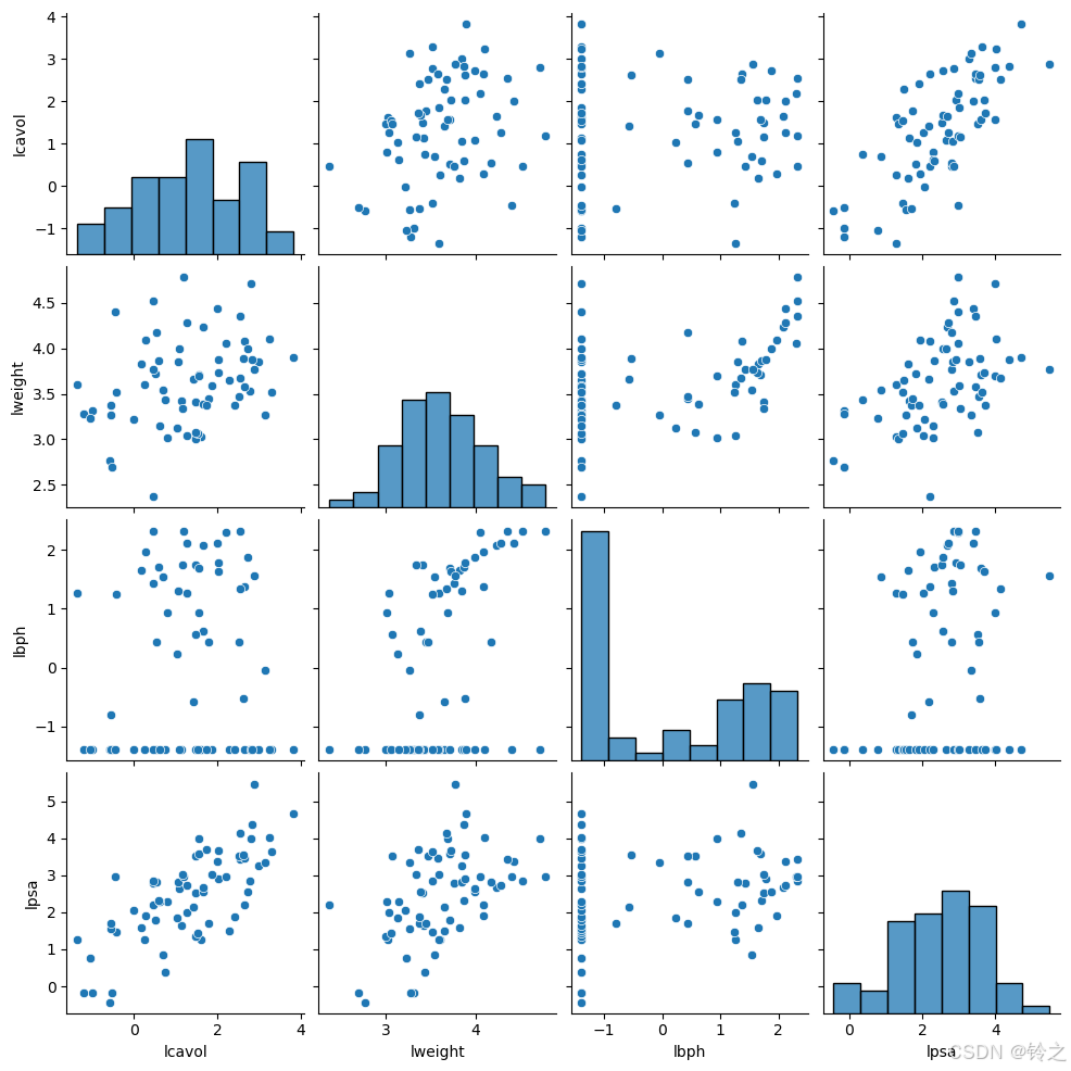
# 散点图矩阵
g=sns.pairplot(train_data.drop(columns=["svi"]))
g.savefig("pairplot_matrix.png", dpi=300, bbox_inches="tight", pad_inches=0)
plt.show()
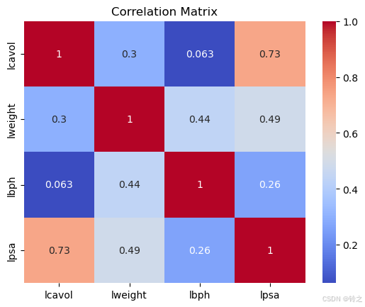
# 计算相关系数矩阵
correlation_matrix = train_data.drop(columns=["svi"]).corr()

# 打印相关系数矩阵
print(correlation_matrix)

# 可视化相关系数矩阵
corr = sns.heatmap(correlation_matrix, annot=true, cmap='coolwarm')
plt.title('correlation matrix')
plt.savefig("correlation_heatmap.png", dpi=300, bbox_inches="tight", pad_inches=0)
# 显示热力图
plt.show()
           lcavol   lweight      lbph      lpsa
lcavol   1.000000  0.300232  0.063168  0.733155
lweight  0.300232  1.000000  0.437042  0.485215
lbph     0.063168  0.437042  1.000000  0.262938
lpsa     0.733155  0.485215  0.262938  1.000000
x, y = train_data.iloc[:, :4], train_data.iloc[:, 4]
x_test, y_test = test_data.iloc[:, :4], test_data.iloc[:, 4]
# (1)多元线性回归,不考虑交互项
reg = linearregression().fit(x, y)
r2=reg.score(x, y)# linearregression模型的score方法计算的是决定系数r2

# 多元线性模型一般计算调整的r2
n_samples = x.shape[0]
n_features = x.shape[1] - 1 if '1' in x.columns else x.shape[1]
adjusted_r2 = 1 - (1-r2)*(n_samples-1)/(n_samples-n_features-1)

print('模型的r2:', r2)
print('模型的调整r2:', adjusted_r2)
模型的r2: 0.6591763372202288
模型的调整r2: 0.6371877138150823
# 查看截距和各变量的回归系数
reg.intercept_, [*zip(x.columns, reg.coef_)]
(-0.3259212340880726,
 [('lcavol', 0.5055208521141417),
  ('lweight', 0.538829197024368),
  ('lbph', 0.14001109982158838),
  ('svi', 0.6718486507008843)])
# 对测试数据集进行预测并查看均方误差mse
y_pred=reg.predict(x_test)
print('在测试数据上的mse:',mean_squared_error(y_test,y_pred)) # 均方误差mse越小越好,最终评价指标

# 也可这样来查看在在训练集上的mse(在sklearn当中,损失使用负数表示,真实值为其相反数)
print('在训练数据上的mse(取负):',cross_val_score(linearregression(), x, y, cv=10, scoring='neg_mean_squared_error').mean())
在测试数据上的mse: 0.45633212204016266
在训练数据上的mse(取负): -0.7466350935712559
#(2)多元线性回归,考虑交互项

poly = polynomialfeatures(degree=2, interaction_only=true, include_bias=false)
x_new = poly.fit_transform(x)
xtest_new=poly.fit_transform(x_test)

# 获取转换后的特征名称
feature_names = poly.get_feature_names_out()

# 将转换后的矩阵转换为dataframe,以便更直观地看到各列对应的特征
df_x_new = pd.dataframe(x_new, columns=feature_names)
df_xtest_new=pd.dataframe(xtest_new, columns=feature_names)
df_x_new.head()
| lcavol | lweight | lbph | svi | lcavol lweight | lcavol lbph | lcavol svi | lweight lbph | lweight svi | lbph svi | |
|---|---|---|---|---|---|---|---|---|---|---|
| 0 | -0.579818 | 2.769459 | -1.386294 | 0.0 | -1.605784 | 0.803799 | -0.0 | -3.839285 | 0.0 | -0.0 |
| 1 | -0.994252 | 3.319626 | -1.386294 | 0.0 | -3.300546 | 1.378326 | -0.0 | -4.601979 | 0.0 | -0.0 |
| 2 | -0.510826 | 2.691243 | -1.386294 | 0.0 | -1.374756 | 0.708155 | -0.0 | -3.730855 | 0.0 | -0.0 |
| 3 | -1.203973 | 3.282789 | -1.386294 | 0.0 | -3.952389 | 1.669061 | -0.0 | -4.550912 | 0.0 | -0.0 |
| 4 | 0.751416 | 3.432373 | -1.386294 | 0.0 | 2.579140 | -1.041684 | 0.0 | -4.758279 | 0.0 | -0.0 |
# 重新进行线性回归
reg = linearregression().fit(df_x_new, y)

# 计算未调整的r^2
r2 = reg.score(df_x_new, y)

# 计算调整的r^2
n_samples = df_x_new.shape[0]
n_features = df_x_new.shape[1] - 1 if '1' in df_x_new.columns else df_x_new.shape[1]
adjusted_r2 = 1 - (1-r2)*(n_samples-1)/(n_samples-n_features-1)

print('模型的r2:', r2)
print('模型的调整r2:', adjusted_r2)
模型的r2: 0.7062588677510526
模型的调整r2: 0.6538050941351692
# 查看截距和各变量的回归系数
reg.intercept_, [*zip(df_x_new.columns, reg.coef_)]
(-0.8829826740678355,
 [('lcavol', 0.75872914094636),
  ('lweight', 0.7239609628400034),
  ('lbph', 1.2336522708050868),
  ('svi', 4.358580417015911),
  ('lcavol lweight', -0.07092260068120437),
  ('lcavol lbph', 0.04191441013906222),
  ('lcavol svi', -0.1955892043514407),
  ('lweight lbph', -0.3007433198540248),
  ('lweight svi', -0.8711274630412957),
  ('lbph svi', -0.21748648070090656)])
# 对测试数据集进行预测并查看均方误差mse
y_pred=reg.predict(df_xtest_new)
print('在测试数据上的mse:',mean_squared_error(y_test,y_pred)) # 均方误差mse越小越好,最终评价指标

# 也可这样来查看在在训练集上的mse(在sklearn当中,损失使用负数表示,真实值为其相反数)
print('在训练数据上的mse(取负):',cross_val_score(linearregression(), df_x_new, y, cv=10, scoring='neg_mean_squared_error').mean())
在测试数据上的mse: 0.5314191336175179
在训练数据上的mse(取负): -1.0443636373693592
由mse可知,这里添加交互项并未有更好的预测结果。
二、线性分类器练习
请对数据集(breast-cancer-wisconsin.txt,来自于 uciml),使用逻辑斯谛回归和 fisher 线性判别设计分类器,实现良性和恶性乳腺癌的分类和预测,给出正确率并对这两种方法做出比较。
附件乳腺癌诊断数据集是699 × 11维的矩阵,11维的特征信息如下。
attribute domain
- sample code number id number
- clump thickness 1 - 10
- uniformity of cell size 1 - 10
- uniformity of cell shape 1 - 10
- marginal adhesion 1 - 10
- single epithelial cell size 1 - 10
- bare nuclei 1 - 10
- bland chromatin 1 - 10
- normal nucleoli 1 - 10
- mitoses 1 - 10
- class: (0 for benign, 1 for malignant)
import pandas as pd
import numpy as np
import matplotlib.pyplot as plt
from sklearn.linear_model import logisticregression
from sklearn.discriminant_analysis import lineardiscriminantanalysis as lda
from sklearn.model_selection import train_test_split, cross_val_score
from sklearn.metrics import accuracy_score, recall_score, roc_auc_score, roc_curve, roc_curve, auc

plt.rcparams["font.sans-serif"]=["simhei"] #设置字体
plt.rcparams["axes.unicode_minus"]=false #该语句解决图像中的“-”负号的乱码问题
data = pd.read_csv('../data/breast-cancer-wisconsin.txt', sep='\t', header=none)
data.drop(data.columns[0], axis=1, inplace=true) # 第一列为id号,对预测无用,删去
data.head()
| 1 | 2 | 3 | 4 | 5 | 6 | 7 | 8 | 9 | 10 | |
|---|---|---|---|---|---|---|---|---|---|---|
| 0 | 5 | 1 | 1 | 1 | 2 | 1 | 3 | 1 | 1 | 0 |
| 1 | 5 | 4 | 4 | 5 | 7 | 10 | 3 | 2 | 1 | 0 |
| 2 | 3 | 1 | 1 | 1 | 2 | 2 | 3 | 1 | 1 | 0 |
| 3 | 6 | 8 | 8 | 1 | 3 | 4 | 3 | 7 | 1 | 0 |
| 4 | 4 | 1 | 1 | 3 | 2 | 1 | 3 | 1 | 1 | 0 |
data.info() # 发现第6列数据类型为object,查看数据后发现是'?',对是问号的位置用这列众数替代
<class 'pandas.core.frame.dataframe'>
rangeindex: 699 entries, 0 to 698
data columns (total 10 columns):
 #   column  non-null count  dtype
---  ------  --------------  -----
 0   1       699 non-null    int64
 1   2       699 non-null    int64
 2   3       699 non-null    int64
 3   4       699 non-null    int64
 4   5       699 non-null    int64
 5   6       699 non-null    object
 6   7       699 non-null    int64
 7   8       699 non-null    int64
 8   9       699 non-null    int64
 9   10      699 non-null    int64
dtypes: int64(9), object(1)
memory usage: 54.7+ kb
data.iloc[:, 5] = data.iloc[:, 5].replace('?', np.nan)
data.iloc[:, 5] = data.iloc[:, 5].fillna(data.iloc[:, 5].mode()[0])
data = data.astype('int64')
data.info()
<class 'pandas.core.frame.dataframe'>
rangeindex: 699 entries, 0 to 698
data columns (total 10 columns):
 #   column  non-null count  dtype
---  ------  --------------  -----
 0   1       699 non-null    int64
 1   2       699 non-null    int64
 2   3       699 non-null    int64
 3   4       699 non-null    int64
 4   5       699 non-null    int64
 5   6       699 non-null    int64
 6   7       699 non-null    int64
 7   8       699 non-null    int64
 8   9       699 non-null    int64
 9   10      699 non-null    int64
dtypes: int64(10)
memory usage: 54.7 kb
# 计算每个类别的样本数量和比例
data.iloc[:,-1].value_counts(),458/(458+241) # 感觉这里不均衡问题还好,不必在意。如严重不均衡需要进行某种处理
(10
 0    458
 1    241
 name: count, dtype: int64,
 0.6552217453505007)
# 划分训练集、测试集
feature_data,target=data.iloc[:,:-1],data.iloc[:,-1]
x, x_test, y, y_test = train_test_split(feature_data,target,test_size=0.2,random_state=2024)
# 逻辑斯谛回归
l1 = []
l2 = []
for i in np.linspace(0.05,3,80):
lrl1 = logisticregression(penalty="l1",solver="liblinear",c=i,max_iter=1000)
lrl2 = logisticregression(penalty="l2",solver="liblinear",c=i,max_iter=1000)
score1=cross_val_score(lrl1,x,y,cv=5).mean()
score2=cross_val_score(lrl2,x,y,cv=5).mean()
l1.append(score1)
l2.append(score2)
# 找到l1和l2中的最大值及其对应的c值
max_l1_score = max(l1)
max_l2_score = max(l2)
c_values=np.linspace(0.05,3,80)
max_l1_c = c_values[l1.index(max_l1_score)]
max_l2_c = c_values[l2.index(max_l2_score)]
# 输出结果
print(f"l1正则化的最大得分为: {max_l1_score}, 对应的c值为: {max_l1_c}")
print(f"l2正则化的最大得分为: {max_l2_score}, 对应的c值为: {max_l2_c}")
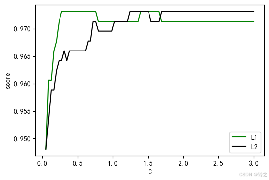
graph = [l1,l2]
color = ["green","black"]
label = ["l1","l2"]
plt.figure(figsize=(6,4))
for i in range(len(graph)):
plt.plot(np.linspace(0.05,3,80),graph[i],color[i],label=label[i])
plt.xlabel('c')
plt.ylabel('score')
plt.legend()
plt.show() # 我们后面采用l2正则化
l1正则化的最大得分为: 0.9731016731016732, 对应的c值为: 0.2740506329113924
l2正则化的最大得分为: 0.9731177606177607, 对应的c值为: 1.2449367088607597
model1 = logisticregression(penalty="l2",solver="liblinear",c=1.2449,max_iter=1000)
model1.fit(x,y)
# 查看训练后的参数
print("模型的权重: ", model1.coef_)
print("模型的截距: ", model1.intercept_)
# 预测测试集
y_pred = model1.predict(x_test)
# 计算准确率
accuracy = accuracy_score(y_test, y_pred)
print(f"准确率: {accuracy}")
# 计算召回率
recall = recall_score(y_test, y_pred)
print(f"召回率: {recall}")
# 预测概率
y_prob = model1.predict_proba(x_test)[:, 1]
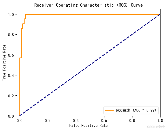
# 计算roc曲线
fpr, tpr, thresholds = roc_curve(y_test, y_prob)
# 计算auc值
roc_auc = auc(fpr, tpr)
# 绘制roc曲线
plt.figure()
plt.plot(fpr, tpr, color='darkorange', lw=2, label=f'roc曲线 (auc = {roc_auc:.2f})')
plt.plot([0, 1], [0, 1], color='navy', lw=2, linestyle='--')
plt.xlim([-0.02, 1.0])
plt.ylim([0.0, 1.05])
plt.xlabel('false positive rate')
plt.ylabel('true positive rate')
plt.title('receiver operating characteristic (roc) curve')
plt.legend(loc="lower right")
plt.show()
模型的权重:  [[ 0.3393932   0.13432484  0.17160089  0.10794074 -0.03199724  0.41146065
   0.27628593  0.13184486  0.23359406]]
模型的截距:  [-6.57189118]
准确率: 0.95
召回率: 0.9047619047619048
fisher线性判别分析(fisher linear discriminant analysis,简称lda)是一种用于分类的降维技术,主要用于在二维或更高维空间中找到最能区分两类数据的投影方向。它的目标是最大化类间距离与类内距离的比率,从而实现最佳的类分离。fisher lda 主要用于以下几个方面:
-
数据降维:将高维数据映射到低维空间,以便于可视化和进一步分析。通常,fisher lda用于将数据从高维空间映射到一维空间。
-
分类:在投影后的低维空间中进行分类,通常在二维空间中可以使用简单的线性分类器(如逻辑回归)进行分类。
fisher lda 的核心概念:
-
类间散布矩阵(between-class scatter matrix):衡量不同类别样本均值之间的散布情况。目标是最大化类间散布矩阵的特征值。
-
类内散布矩阵(within-class scatter matrix):衡量同一类别样本之间的散布情况。目标是最小化类内散布矩阵的特征值。
-
优化目标:通过找到一个投影方向,使得在该方向上,类间散布最大化,类内散布最小化。这个目标可以通过求解广义瑞利商(rayleigh quotient)来实现。
fisher lda 的数学推导:
-
定义:
-
类内散布矩阵 s w s_w sw:
s w = ∑ i = 1 c ∑ x ∈ class i ( x − μ i ) ( x − μ i ) t s_w = \sum_{i=1}^c \sum_{x \in \text{class}_i} (x - \mu_i)(x - \mu_i)^t sw=i=1∑cx∈classi∑(x−μi)(x−μi)t
其中, μ i \mu_i μi 是类别 i i i 的均值, c c c 是类别的总数。 -
类间散布矩阵 s b s_b sb:
s b = ∑ i = 1 c n i ( μ i − μ ) ( μ i − μ ) t s_b = \sum_{i=1}^c n_i (\mu_i - \mu)(\mu_i - \mu)^t sb=i=1∑cni(μi−μ)(μi−μ)t
其中, μ \mu μ 是所有样本的整体均值, n i n_i ni 是类别 i i i 的样本数量。
-
-
目标:
- 寻找投影向量
w
w
w 使得:
j ( w ) = w t s b w w t s w w j(w) = \frac{w^t s_b w}{w^t s_w w} j(w)=wtswwwtsbw
最大化目标函数 j ( w ) j(w) j(w)。
- 寻找投影向量
w
w
w 使得:
-
求解:
- 求解广义特征值问题: s b w = λ s w w s_b w = \lambda s_w w sbw=λsww,得到特征值 λ \lambda λ 和特征向量 w w w。
- 选择最大特征值对应的特征向量作为最终的投影方向。
fisher lda 的应用场景:
- 模式识别:例如在图像识别中,通过lda将图像数据从高维空间映射到低维空间,从而提高分类效率。
- 生物统计学:在基因表达数据分析中,通过lda减少维度以提高分类准确率。
- 金融分析:在金融数据分析中,使用lda进行风险分类或预测。
fisher lda 适用于线性可分的数据集,特别是在类别之间有明显的分隔时表现良好。如果数据集的类别非常复杂或者非线性,可能需要结合其他方法或算法进行更精确的分类。
# 线性判别分析

# 初始化lda模型
lda = lda()

# 训练lda模型
lda.fit(x, y)

# 打印训练参数
print("lda coefficients:")
print(lda.coef_)
print("lda intercept:")
print(lda.intercept_)
print("lda explained variance ratio:")
print(lda.explained_variance_ratio_)

# 进行预测
y_pred = lda.predict(x_test)

# 计算准确率和召回率
accuracy = accuracy_score(y_test, y_pred)
recall = recall_score(y_test, y_pred)
print("accuracy:", accuracy)
print("recall:", recall)

# 计算roc曲线
decision_function = lda.decision_function(x_test)
fpr, tpr, thresholds = roc_curve(y_test, y_prob)

# 计算auc值
roc_auc = auc(fpr, tpr)

# 绘制roc曲线
plt.figure()
plt.plot(fpr, tpr, color='darkorange', lw=2, label=f'roc曲线 (auc = {roc_auc:.2f})')
plt.plot([0, 1], [0, 1], color='navy', lw=2, linestyle='--')
plt.xlim([-0.02, 1.0])
plt.ylim([0.0, 1.05])
plt.xlabel('false positive rate')
plt.ylabel('true positive rate')
plt.title('receiver operating characteristic (roc) curve')
plt.legend(loc="lower right")
plt.show()
lda coefficients:
[[1.06086642 0.51731242 0.37722528 0.09113927 0.25333371 1.32065688
  0.7728181  0.4409523  0.21131264]]
lda intercept:
[-21.72114264]
lda explained variance ratio:
[1.]
accuracy: 0.95
recall: 0.9047619047619048

lda.predict(x_test)==model1.predict(x_test) # 难怪图像一模一样
array([ true,  true,  true,  true,  true,  true,  true,  true,  true,
        true,  true,  true,  true,  true,  true,  true,  true,  true,
        true,  true,  true,  true,  true,  true,  true,  true,  true,
        true,  true,  true,  true,  true,  true,  true,  true,  true,
        true,  true,  true,  true,  true,  true,  true,  true,  true,
        true,  true,  true,  true,  true,  true,  true,  true,  true,
        true,  true,  true,  true,  true,  true,  true,  true,  true,
        true,  true,  true,  true,  true,  true,  true,  true,  true,
        true,  true,  true,  true,  true,  true,  true,  true,  true,
        true,  true,  true,  true,  true,  true,  true,  true,  true,
        true,  true,  true,  true,  true,  true,  true,  true,  true,
        true,  true,  true,  true,  true,  true,  true,  true,  true,
        true,  true,  true,  true,  true,  true,  true,  true,  true,
        true,  true,  true,  true,  true,  true,  true,  true,  true,
        true,  true,  true,  true,  true,  true,  true,  true,  true,
        true,  true,  true,  true,  true])
`

发表评论