c#基于scottplot进行可视化
前言
上一篇文章跟大家分享了用numsharp实现简单的线性回归,但是没有进行可视化,可能对拟合的过程没有直观的感受,因此今天跟大家介绍一下使用c#基于scottplot进行可视化,当然python的代码,我也会同步进行可视化。
python代码进行可视化
python代码用matplotlib做了可视化,我就不具体介绍了。
修改之后的python代码如下:
#the optimal values of m and b can be actually calculated with way less effort than doing a linear regression.
#this is just to demonstrate gradient descent

import numpy as np
import matplotlib.pyplot as plt
from matplotlib.animation import funcanimation


# y = mx + b
# m is slope, b is y-intercept
def compute_error_for_line_given_points(b, m, points):
    totalerror = 0
    for i in range(0, len(points)):
        x = points[i, 0]
        y = points[i, 1]
        totalerror += (y - (m * x + b)) ** 2
    return totalerror / float(len(points))

def step_gradient(b_current, m_current, points, learningrate):
    b_gradient = 0
    m_gradient = 0
    n = float(len(points))
    for i in range(0, len(points)):
        x = points[i, 0]
        y = points[i, 1]
        b_gradient += -(2/n) * (y - ((m_current * x) + b_current))
        m_gradient += -(2/n) * x * (y - ((m_current * x) + b_current))
    new_b = b_current - (learningrate * b_gradient)
    new_m = m_current - (learningrate * m_gradient)
    return [new_b, new_m]

def gradient_descent_runner(points, starting_b, starting_m, learning_rate, num_iterations):
    b = starting_b
    m = starting_m
    args_data = []
    for i in range(num_iterations):
        b, m = step_gradient(b, m, np.array(points), learning_rate)
        args_data.append((b,m))
    return args_data

if __name__ == '__main__':
     points = np.genfromtxt("data.csv", delimiter=",")
     learning_rate = 0.0001
     initial_b = 0 # initial y-intercept guess
     initial_m = 0 # initial slope guess
     num_iterations = 10
     print ("starting gradient descent at b = {0}, m = {1}, error = {2}".format(initial_b, initial_m, compute_error_for_line_given_points(initial_b, initial_m, points)))
     print ("running...")
     args_data = gradient_descent_runner(points, initial_b, initial_m, learning_rate, num_iterations)

     b = args_data[-1][0]
     m = args_data[-1][1]

     print ("after {0} iterations b = {1}, m = {2}, error = {3}".format(num_iterations, b, m, compute_error_for_line_given_points(b, m, points)))

     data = np.array(points).reshape(100,2)
     x1 = data[:,0]
     y1 = data[:,1]

     x2 = np.linspace(20, 80, 100)
     y2 = initial_m * x2 + initial_b

     data2 = np.array(args_data)
     b_every = data2[:,0]
     m_every = data2[:,1]

     # 创建图形和轴
     fig, ax = plt.subplots()
     line1, = ax.plot(x1, y1, 'ro')
     line2, = ax.plot(x2,y2)

     # 添加标签和标题
     plt.xlabel('x')
     plt.ylabel('y')
     plt.title('graph of y = mx + b')

     # 添加网格
     plt.grid(true)

    # 定义更新函数
     def update(frame):
        line2.set_ydata(m_every[frame] * x2 + b_every[frame])
        ax.set_title(f'{frame} graph of y = {m_every[frame]:.2f}x + {b_every[frame]:.2f}')

# 创建动画
animation = funcanimation(fig, update, frames=len(data2), interval=500)

# 显示动画
plt.show()
实现的效果如下所示:


c#代码进行可视化
这是本文重点介绍的内容,本文的c#代码通过scottplot进行可视化。
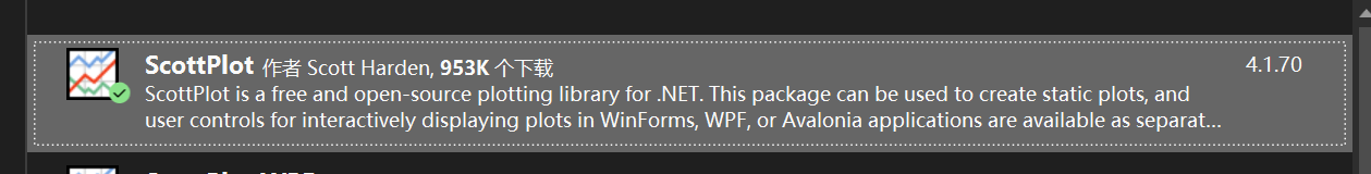
scottplot简介
scottplot 是一个免费的开源绘图库,用于 .net,可以轻松以交互方式显示大型数据集。
控制台程序可视化
首先我先介绍一下在控制台程序中进行可视化。
首先添加scottplot包:
将上篇文章中的c#代码修改如下:
using numsharp;

namespace linearregressiondemo
{
    internal class program
    {
        static void main(string[] args)
        {
            //创建double类型的列表
            list<double> array = new list<double>();
            list<double> argslist = new list<double>();

            // 指定csv文件的路径
            string filepath = "你的data.csv路径";

            // 调用readcsv方法读取csv文件数据
            array = readcsv(filepath);

            var array = np.array(array).reshape(100,2);

            double learning_rate = 0.0001;
            double initial_b = 0;
            double initial_m = 0;
            double num_iterations = 10;

            console.writeline($"starting gradient descent at b = {initial_b}, m = {initial_m}, error = {compute_error_for_line_given_points(initial_b, initial_m, array)}");
            console.writeline("running...");
            argslist = gradient_descent_runner(array, initial_b, initial_m, learning_rate, num_iterations);
            double b = argslist[argslist.count - 2];
            double m = argslist[argslist.count - 1];
            console.writeline($"after {num_iterations} iterations b = {b}, m = {m}, error = {compute_error_for_line_given_points(b, m, array)}");
            console.readline();

            var x1 = array[$":", 0];
            var y1 = array[$":", 1];
            var y2 = m * x1 + b;

            scottplot.plot myplot = new(400, 300);
            myplot.addscatterpoints(x1.toarray<double>(), y1.toarray<double>(), markersize: 5);
            myplot.addscatter(x1.toarray<double>(), y2.toarray<double>(), markersize: 0);
            myplot.title($"y = {m:0.00}x + {b:0.00}");

            myplot.savefig("图片.png");

        }

        static list<double> readcsv(string filepath)
        {
            list<double> array = new list<double>();
            try
            {
                // 使用file.readalllines读取csv文件的所有行
                string[] lines = file.readalllines(filepath);

                // 遍历每一行数据
                foreach (string line in lines)
                {
                    // 使用逗号分隔符拆分每一行的数据
                    string[] values = line.split(',');

                    // 打印每一行的数据
                    foreach (string value in values)
                    {
                        array.add(convert.todouble(value));
                    }
                }
            }
            catch (exception ex)
            {
                console.writeline("发生错误: " + ex.message);
            }
            return array;
        }

        public static double compute_error_for_line_given_points(double b,double m,ndarray array)
        {
            double totalerror = 0;
            for(int i = 0;i < array.shape[0];i++)
            {
                double x = array[i, 0];
                double y = array[i, 1];
                totalerror += math.pow((y - (m*x+b)),2);
            }
            return totalerror / array.shape[0];
        }

        public static double[] step_gradient(double b_current,double m_current,ndarray array,double learningrate)
        {
            double[] args = new double[2];
            double b_gradient = 0;
            double m_gradient = 0;
            double n = array.shape[0];

            for (int i = 0; i < array.shape[0]; i++)
            {
                double x = array[i, 0];
                double y = array[i, 1];
                b_gradient += -(2 / n) * (y - ((m_current * x) + b_current));
                m_gradient += -(2 / n) * x * (y - ((m_current * x) + b_current));
            }

            double new_b = b_current - (learningrate * b_gradient);
            double new_m = m_current - (learningrate * m_gradient);
            args[0] = new_b;
            args[1] = new_m;

            return args;
        }

        public static list<double> gradient_descent_runner(ndarray array, double starting_b, double starting_m, double learningrate,double num_iterations)
        {
            double[] args = new double[2];
            list<double> argslist = new list<double>();
            args[0] = starting_b;
            args[1] = starting_m;

            for(int i = 0 ; i < num_iterations; i++)
            {
                args = step_gradient(args[0], args[1], array, learningrate);
                argslist.addrange(args);
            }

            return argslist;
        }


    }
}
然后得到的图片如下所示:

在以上代码中需要注意的地方:
  var x1 = array[$":", 0];
  var y1 = array[$":", 1];
是在使用numsharp中的切片,x1表示所有行的第一列,y1表示所有行的第二列。
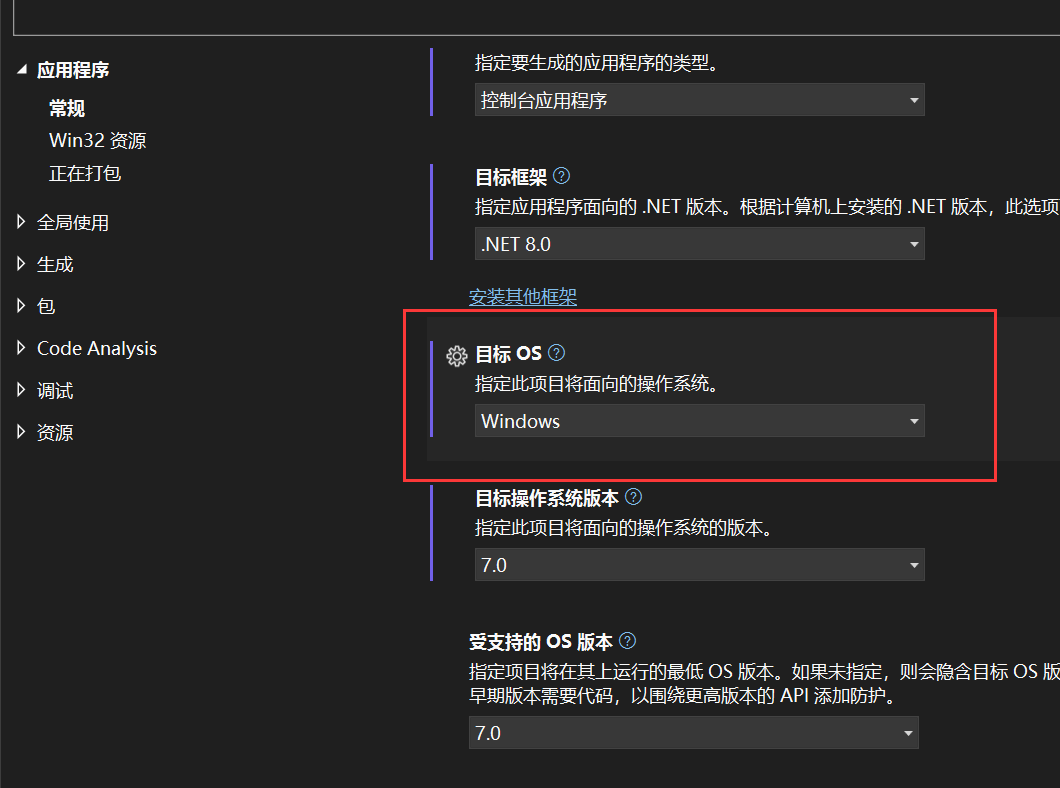
当然我们不满足于只是保存图片,在控制台应用程序中,再添加一个 scottplot.winforms包:

右键控制台项目选择属性,将目标os改为windows:
将上述代码中的
myplot.savefig("图片.png");
修改为:
 var viewer = new scottplot.formsplotviewer(myplot);
 viewer.showdialog();
再次运行结果如下:

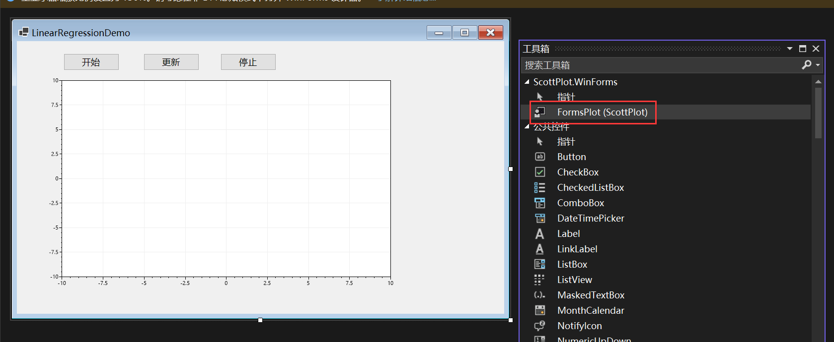
winform进行可视化
我也想像python代码中那样画动图,因此做了个winform程序进行演示。
首先创建一个winform,添加scottplot.winforms包,然后从工具箱中添加formsplot这个控件:
有两种方法实现,第一种方法用了定时器:
using numsharp;
namespace winformdemo
{
    public partial class form1 : form
    {
        system.windows.forms.timer updatetimer = new system.windows.forms.timer();
        int num_iterations;
        int count = 0;
        ndarray? x1, y1, b_each, m_each;
        public form1()
        {
            initializecomponent();
        }

        private void button1_click(object sender, eventargs e)
        {
            startlinearregression();
        }

        public void startlinearregression()
        {
            //创建double类型的列表
            list<double> array = new list<double>();
            list<double> argslist = new list<double>();

            // 指定csv文件的路径
            string filepath = "你的data.csv路径";

            // 调用readcsv方法读取csv文件数据
            array = readcsv(filepath);

            var array = np.array(array).reshape(100, 2);

            double learning_rate = 0.0001;
            double initial_b = 0;
            double initial_m = 0;
            num_iterations = 10;

            argslist = gradient_descent_runner(array, initial_b, initial_m, learning_rate, num_iterations);

            x1 = array[$":", 0];
            y1 = array[$":", 1];

            var argsarr = np.array(argslist).reshape(num_iterations, 2);
            b_each = argsarr[$":", 0];
            m_each = argsarr[$":", 1];

            double b = b_each[-1];
            double m = m_each[-1];
            var y2 = m * x1 + b;

            formsplot1.plot.addscatterpoints(x1.toarray<double>(), y1.toarray<double>(), markersize: 5);
            //formsplot1.plot.addscatter(x1.toarray<double>(), y2.toarray<double>(), markersize: 0);
            formsplot1.render();


        }

        static list<double> readcsv(string filepath)
        {
            list<double> array = new list<double>();
            try
            {
                // 使用file.readalllines读取csv文件的所有行
                string[] lines = file.readalllines(filepath);

                // 遍历每一行数据
                foreach (string line in lines)
                {
                    // 使用逗号分隔符拆分每一行的数据
                    string[] values = line.split(',');

                    // 打印每一行的数据
                    foreach (string value in values)
                    {
                        array.add(convert.todouble(value));
                    }
                }
            }
            catch (exception ex)
            {
                console.writeline("发生错误: " + ex.message);
            }
            return array;
        }

        public static double compute_error_for_line_given_points(double b, double m, ndarray array)
        {
            double totalerror = 0;
            for (int i = 0; i < array.shape[0]; i++)
            {
                double x = array[i, 0];
                double y = array[i, 1];
                totalerror += math.pow((y - (m * x + b)), 2);
            }
            return totalerror / array.shape[0];
        }

        public static double[] step_gradient(double b_current, double m_current, ndarray array, double learningrate)
        {
            double[] args = new double[2];
            double b_gradient = 0;
            double m_gradient = 0;
            double n = array.shape[0];

            for (int i = 0; i < array.shape[0]; i++)
            {
                double x = array[i, 0];
                double y = array[i, 1];
                b_gradient += -(2 / n) * (y - ((m_current * x) + b_current));
                m_gradient += -(2 / n) * x * (y - ((m_current * x) + b_current));
            }

            double new_b = b_current - (learningrate * b_gradient);
            double new_m = m_current - (learningrate * m_gradient);
            args[0] = new_b;
            args[1] = new_m;

            return args;
        }

        public static list<double> gradient_descent_runner(ndarray array, double starting_b, double starting_m, double learningrate, double num_iterations)
        {
            double[] args = new double[2];
            list<double> argslist = new list<double>();
            args[0] = starting_b;
            args[1] = starting_m;

            for (int i = 0; i < num_iterations; i++)
            {
                args = step_gradient(args[0], args[1], array, learningrate);
                argslist.addrange(args);
            }

            return argslist;
        }

        private void button2_click(object sender, eventargs e)
        {
            // 初始化定时器
            updatetimer.interval = 1000; // 设置定时器触发间隔(毫秒)
            updatetimer.tick += updatetimer_tick;
            updatetimer.start();
        }

        private void updatetimer_tick(object? sender, eventargs e)
        {
            if (count >= num_iterations)
            {
                updatetimer.stop();
            }
            else
            {
                updateplot(count);
            }

            count++;
        }

        public void updateplot(int count)
        {

            double b = b_each?[count];
            double m = m_each?[count];

            var y2 = m * x1 + b;

            formsplot1.plot.clear();
            formsplot1.plot.addscatterpoints(x1?.toarray<double>(), y1?.toarray<double>(), markersize: 5);
            formsplot1.plot.addscatter(x1?.toarray<double>(), y2.toarray<double>(), markersize: 0);
            formsplot1.plot.title($"第{count + 1}次迭代:y = {m:0.00}x + {b:0.00}");
            formsplot1.render();
        }

        private void button3_click(object sender, eventargs e)
        {
            updatetimer.stop();
        }

        private void form1_load(object sender, eventargs e)
        {

        }
    }
}
简单介绍一下思路,首先创建list<double> argslist用来保存每次迭代生成的参数b、m,然后用
var argsarr = np.array(argslist).reshape(num_iterations, 2);
将argslist通过np.array()方法转化为ndarray,然后再调用reshape方法,转化成行数等于迭代次数,列数为2,即每一行对应一组参数值b、m。
            b_each = argsarr[$":", 0];
            m_each = argsarr[$":", 1];
argsarr[$":", 0]表示每一行中第一列的值,也就是每一个b,argsarr[$":", 1]表示每一行中第二列的值。
            double b = b_each[-1];
            double m = m_each[-1];
b_each[-1]用了numsharp的功能表示b_each最后一个元素。
实现效果如下所示:


另一种方法可以通过异步实现:
using numsharp;

namespace winformdemo
{
    public partial class form2 : form
    {
        int num_iterations;
        ndarray? x1, y1, b_each, m_each;
        public form2()
        {
            initializecomponent();
        }

        private void button1_click(object sender, eventargs e)
        {
            startlinearregression();
        }

        public void startlinearregression()
        {
            //创建double类型的列表
            list<double> array = new list<double>();
            list<double> argslist = new list<double>();

            // 指定csv文件的路径
            string filepath = "你的data.csv路径";

            // 调用readcsv方法读取csv文件数据
            array = readcsv(filepath);

            var array = np.array(array).reshape(100, 2);

            double learning_rate = 0.0001;
            double initial_b = 0;
            double initial_m = 0;
            num_iterations = 10;

            argslist = gradient_descent_runner(array, initial_b, initial_m, learning_rate, num_iterations);

            x1 = array[$":", 0];
            y1 = array[$":", 1];

            var argsarr = np.array(argslist).reshape(num_iterations, 2);
            b_each = argsarr[$":", 0];
            m_each = argsarr[$":", 1];

            double b = b_each[-1];
            double m = m_each[-1];
            var y2 = m * x1 + b;

            formsplot1.plot.addscatterpoints(x1.toarray<double>(), y1.toarray<double>(), markersize: 5);
            formsplot1.render();
        }

        static list<double> readcsv(string filepath)
        {
            list<double> array = new list<double>();
            try
            {
                // 使用file.readalllines读取csv文件的所有行
                string[] lines = file.readalllines(filepath);

                // 遍历每一行数据
                foreach (string line in lines)
                {
                    // 使用逗号分隔符拆分每一行的数据
                    string[] values = line.split(',');

                    // 打印每一行的数据
                    foreach (string value in values)
                    {
                        array.add(convert.todouble(value));
                    }
                }
            }
            catch (exception ex)
            {
                console.writeline("发生错误: " + ex.message);
            }
            return array;
        }

        public static double compute_error_for_line_given_points(double b, double m, ndarray array)
        {
            double totalerror = 0;
            for (int i = 0; i < array.shape[0]; i++)
            {
                double x = array[i, 0];
                double y = array[i, 1];
                totalerror += math.pow((y - (m * x + b)), 2);
            }
            return totalerror / array.shape[0];
        }

        public static double[] step_gradient(double b_current, double m_current, ndarray array, double learningrate)
        {
            double[] args = new double[2];
            double b_gradient = 0;
            double m_gradient = 0;
            double n = array.shape[0];

            for (int i = 0; i < array.shape[0]; i++)
            {
                double x = array[i, 0];
                double y = array[i, 1];
                b_gradient += -(2 / n) * (y - ((m_current * x) + b_current));
                m_gradient += -(2 / n) * x * (y - ((m_current * x) + b_current));
            }

            double new_b = b_current - (learningrate * b_gradient);
            double new_m = m_current - (learningrate * m_gradient);
            args[0] = new_b;
            args[1] = new_m;

            return args;
        }

        public static list<double> gradient_descent_runner(ndarray array, double starting_b, double starting_m, double learningrate, double num_iterations)
        {
            double[] args = new double[2];
            list<double> argslist = new list<double>();
            args[0] = starting_b;
            args[1] = starting_m;

            for (int i = 0; i < num_iterations; i++)
            {
                args = step_gradient(args[0], args[1], array, learningrate);
                argslist.addrange(args);
            }

            return argslist;
        }

        private void form2_load(object sender, eventargs e)
        {

        }

        public async task updategraph()
        {
            for (int i = 0; i < num_iterations; i++)
            {
                double b = b_each?[i];
                double m = m_each?[i];
                var y2 = m * x1 + b;

                formsplot1.plot.clear();
                formsplot1.plot.addscatterpoints(x1?.toarray<double>(), y1?.toarray<double>(), markersize: 5);
                formsplot1.plot.addscatter(x1?.toarray<double>(), y2.toarray<double>(), markersize: 0);
                formsplot1.plot.title($"第{i + 1}次迭代:y = {m:0.00}x + {b:0.00}");
                formsplot1.render();

                await task.delay(1000);
            }


        }

        private async void button2_click(object sender, eventargs e)
        {
            await updategraph();
        }
    }
}
点击更新按钮开始执行异步任务:
 private async void button2_click(object sender, eventargs e)
        {
            await updategraph();
        }
 public async task updategraph()
        {
            for (int i = 0; i < num_iterations; i++)
            {
                double b = b_each?[i];
                double m = m_each?[i];
                var y2 = m * x1 + b;

                formsplot1.plot.clear();
                formsplot1.plot.addscatterpoints(x1?.toarray<double>(), y1?.toarray<double>(), markersize: 5);
                formsplot1.plot.addscatter(x1?.toarray<double>(), y2.toarray<double>(), markersize: 0);
                formsplot1.plot.title($"第{i + 1}次迭代:y = {m:0.00}x + {b:0.00}");
                formsplot1.render();

                await task.delay(1000);
            }
实现效果如下:


总结
本文以一个控制台应用与一个winform程序为例向大家介绍了c#如何基于scottplot进行数据可视化,并介绍了实现动态绘图的两种方式,一种是使用定时器,另一种是使用异步操作,希望对你有所帮助。


发表评论