Python实现网格交易策略的过程_Python

网格交易是一种经典的量化交易策略，其核心思想是在价格上下预设多个“网格”，当价格触发特定网格时执行买入或卖出操作，以低买高卖赚取区间波动收益。

最近开始接触python量化交易，记录一个简单的策略实现和回测的完整框架，不包含实盘。

量化框架是ccxt和backtrader。backtrader用来做策略和回测，ccxt用来调用交易所的api用来获取数据或日后的实盘。ccxt主要是用来调加密货币交易所的，因为现在加密货币对量化比较友好，首先它获取数据就比传统的股票方便，直接调交易所的api就行，甚至不需要注册账号，我之前看过很多股票的量化教程，获取数据还是比较有门槛的。其次他是7x24小时全年无休的，交易也比较方便。

好的接下来进入正题，看看我们的第一个量化策略是怎么实现的吧。

我们使用的网格交易策略，是一种基于市场波动的自动化交易策略，核心逻辑是通过在特定价格区间内设置一系列 “网格节点”，当价格波动触及节点时自动执行买入或卖出操作，利用价格的上下震荡实现 “低买高卖” 的循环获利。其本质是将市场波动转化为盈利机会，尤其适合震荡行情。风险就是在持续向下的行情可能在高网格持续买入，越跌越买导致资金耗尽。

下面是策略的实现，继承bt.strategy，策略的执行放在next函数中。

import backtrader as bt
import math
# 1. 网格策略核心类
class gridstrategy(bt.strategy):
    params = (
        ('number', 10),  # 网格总数
        ('open_percent', 0.5),  # 初始建仓比例(50%)
        ('distance', 0.01),  # 网格间距(1%)
        ('base_price', 5.0)  # 基准价格
    )
    def __init__(self):
        self.open_flag = false  # 初始建仓标记
        self.last_index = 0  # 上次网格位置
        self.per_size = 0  # 每格交易量
        self.max_index = 0  # 网格上边界
        self.min_index = 0  # 网格下边界
    def next(self):
        # 初始建仓逻辑（价格接近基准价时触发）
        if not self.open_flag and math.fabs(self.data.close[0] - self.p.base_price) / self.p.base_price < 0.01:
            # 计算初始仓位（50%资金）
            buy_size = self.broker.getvalue() * self.p.open_percent / self.data.close[0]
            self.buy(size=buy_size)
            # 初始化网格参数
            self.last_index = 0
            self.per_size = self.broker.getvalue() / self.data.close[0] / self.p.number
            self.max_index = int(self.p.number * self.p.open_percent)
            self.min_index = -int(self.p.number * (1 - self.p.open_percent))
            self.open_flag = true
        # 网格调仓逻辑
        if self.open_flag:
            # 计算当前网格位置（按间距归一化）
            current_index = int((self.data.close[0] - self.p.base_price) / self.p.distance)
            # 边界保护（防止破网）
            current_index = max(min(current_index, self.max_index), self.min_index)
            # 网格变化时交易
            change = current_index - self.last_index
            if change > 0:  # 价格上涨→卖出
                self.sell(size=abs(change) * self.per_size)
            elif change < 0:  # 价格下跌→买入
                self.buy(size=abs(change) * self.per_size)
            self.last_index = current_index  # 更新网格位置
    # 2. 订单状态跟踪（调试用）
    def notify_order(self, order):
        if order.status in [order.completed]:
            action = '买入' if order.isbuy() else '卖出'
            print(f'{action}成交: 价格={order.executed.price:.2f}, 数量={order.executed.size}')

然后在另一个脚本中使用这个策略：

import backtrader as bt
from gridstrategy import gridstrategy
from backtrader.feeds import pandasdata
import ccxt
import pandas as pd
# 连接交易所（以币安为例）
exchange = ccxt.binance({
    'enableratelimit': true,  # 启用频率限制[6](@ref)
    'options': {'defaulttype': 'spot'}  # 现货数据
})
# 获取eth/usdt历史k线（1小时周期）
def fetch_eth_data(days=30, timeframe='1h'):
    since = exchange.parse8601((pd.timestamp.utcnow() - pd.timedelta(days=days)).isoformat())
    ohlcv = exchange.fetch_ohlcv('eth/usdt', timeframe, since=since)
    df = pd.dataframe(ohlcv, columns=['timestamp', 'open', 'high', 'low', 'close', 'volume'])
    df['timestamp'] = pd.to_datetime(df['timestamp'], unit='ms')
    df.set_index('timestamp', inplace=true)
    return df
eth_data = fetch_eth_data(days=90, timeframe='1h')  # 获取90天1小时数据
print(eth_data)
class ccxtdata(pandasdata):
    lines = ('volume',)  # 声明额外数据列
    params = (
        ('datetime', none),  # 使用索引作为时间列
        ('open', 'open'),
        ('high', 'high'),
        ('low', 'low'),
        ('close', 'close'),
        ('volume', 'volume'),
    )
# 数据实例化
data_feed = ccxtdata(dataname=eth_data)
# 初始化引擎
cerebro = bt.cerebro()
cerebro.addstrategy(
    gridstrategy,
    base_price=1803.70,  # 设置标的基准价
    distance=10,  # 网格间距5%（按价格波动调整）
    number=100  # 增加网格密度
)
cerebro.adddata(data_feed)
cerebro.broker.setcash(10000.0)  # 初始资金
cerebro.broker.setcommission(commission=0.001)  # 手续费0.1%[3](@ref)
# 运行回测
print('初始资金:', cerebro.broker.getvalue())
cerebro.run()
print('最终资金:', cerebro.broker.getvalue())
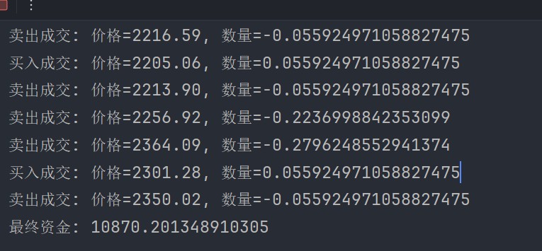
# 可视化结果
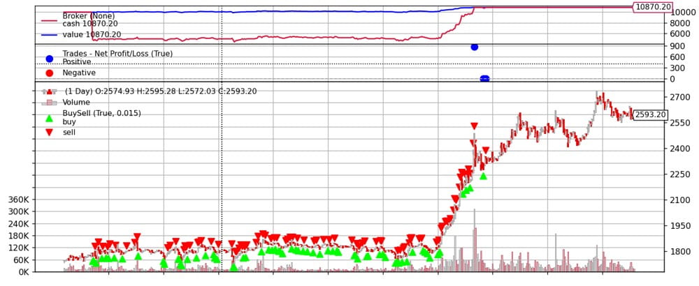
cerebro.plot(style='candlestick')

执行上面的脚本，可以看到回测结果，我们投入10000块，经过差不多一个月的时间最终受益有870块之多，实在是太赚了xd。