【动手学深度学习】深入浅出深度学习之利用神经网络识别螺旋状数据集

目录

🌞一、实验目的

🌞二、实验准备

🌞三、实验内容

🌼1. 生成螺旋状数据集

🌼2. 打印数据集

🌼3. 编程实现

🌻仿射层-affine类

🌻传播层-sigmoid类

🌻损失函数相关类

🌻三层神经网络类-threelayernet

🌻随机梯度下降法的类-sgd

🌻训练过程

🌻绘制迭代效果图

🌞四、实验心得

🌞一、实验目的

1. 利用神经网络识别螺旋状数据集（python实现）；
2. 正确理解深度学习所需的数学知识。

🌞二、实验准备

1. 根据gpu安装pytorch版本实现gpu运行实验代码；
2. 配置环境用来运行 python、jupyter notebook和相关库等相关库。

🌞三、实验内容

资源获取：关注公众号【科创视野】回复  深度学习

🌼1. 生成螺旋状数据集

（1）利用numpy库生成螺旋状数据集，python源码如下：

# coding: utf-8
import numpy as np


def load_data(seed=2020264):   #🍕🍕🍕生成数据集🍕🍕🍕
    np.random.seed(seed)  #设置随机数种子
    n = 100  # 各类的样本数
    dim = 2  # 数据的元素个数
    cls_num = 3  # 类别数

    x = np.zeros((n*cls_num, dim))
    t = np.zeros((n*cls_num, cls_num), dtype=np.int)

    for j in range(cls_num):
        for i in range(n):#n*j, n*(j+1)):
            rate = i / n
            radius = 1.0*rate
            theta = j*4.0 + 4.0*rate + np.random.randn()*0.2

            ix = n*j + i
            x[ix] = np.array([radius*np.sin(theta),
                              radius*np.cos(theta)]).flatten()
            t[ix, j] = 1

    return x, t

解释：

🌼2. 打印数据集

在加载完数据集后，利用plt将生成的数据集打印出来，python源码如下：

# coding: utf-8
import sys
sys.path.append('..')  # 为了引入父目录的文件而进行的设定
import matplotlib.pyplot as plt


x, t = load_data()
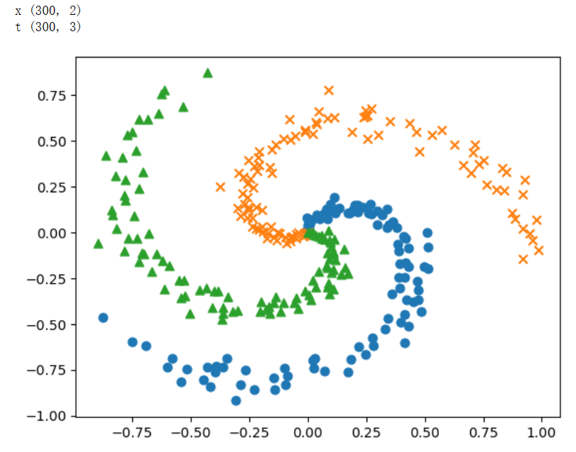
print('x', x.shape)  # (300, 2)
print('t', t.shape)  # (300, 3)

# 绘制数据点
n = 100
cls_num = 3
markers = ['o', 'x', '^']
for i in range(cls_num):
    plt.scatter(x[i*n:(i+1)*n, 0], x[i*n:(i+1)*n, 1], s=40, marker=markers[i])
plt.show()

解释：

结果图为：

🌼3. 编程实现

🌻仿射层-affine类

class affine:
    def __init__(self,w,b):
        self.params = [w,b]#保存参数
        self.grads = [np.zeros_like(w),np.zeros_like(b)]#保存梯度
        self.x = none
    def forward(self,x):
        w,b = self.params
        out = np.dot(x,w) + b
        self.x = x
        return out
    def backward(self,dout):
        w,b = self.params
        dx = np.dot(dout,w.t)
        dw = np.dot(self.x.t,dout)
        db = np.sum(dout,axis=0)
        
        self.grads[0][...] = dw  
        self.grads[1][...] = db
        return dx

解释：

🌻传播层-sigmoid类

class sigmoid:
    def __init__(self):
        self.params = []
        self.grads = []
        self.out = none
    def forward(self,x):
        out = 1 / (1 + np.exp(-x))
        self.out = out
        return out
    def backward(self,dout):
        dx = dout * (1.0 - self.out) * self.out
        return dx

解释：

🌻损失函数相关类

def softmax(x):
    if x.ndim == 1:
        x = x - np.max(x)
        x = np.exp(x)/np.sum(np.exp(x))
    elif x.ndim == 2:
        x = x - x.max(axis = 1,keepdims = true)
        x = np.exp(x)
        x /= x.sum(axis=1, keepdims=true)
    return x

def cross_entropy_error(y,t):
    if y.ndim == 1:
        t = t.reshape(1,t.size)
        y = y.reshape(1,y.size)
        
    #因为监督标签是one-hot-vector形式，所以这里要取下标    
    if t.size == y.size:
        t = t.argmax(dim=1)
    
    batch_size = y.shape[0]
    #没看懂为啥
    return -np.sum(np.log(y[np.arange(batch_size), t] + 1e-7)) / batch_size
    
    
class softmaxwithloss:
    def __init__(self):
        self.params = []
        self.grads = []
        self.y = none #softmx的输出
        self.t = none #监督标签
    
    def forward(self,x,t):
        self.t = t
        self.y = softmax(x)
        
        if self.t.size == self.y.size:
            self.t = self.t.argmax(axis=1)
        
        loss = cross_entropy_error(self.y,self.t)
        return loss
    def backward(self,dout =1):
        batch_size = self.t.shape[0]
        dx = self.y.copy()
        dx[np.arange(batch_size),self.t] -= 1
        dx *= dout
        dx = dx/batch_size
        
        return dx

解释：

🌻三层神经网络类-threelayernet

class threelayernet:
    def __init__(self,input_size,hidden_size1,hidden_size2,output_size):
        i,h1,h2,o = input_size,hidden_size1,hidden_size2,output_size
    #初始化权重和偏置
        w1 = 0.01 * np.random.randn(i,h1)    #形状：i*h
        b1 = np.zeros(h1)
        w2 = 0.01 * np.random.randn(h1,h2)
        b2 = np.zeros(h2)
        w3 = 0.01 * np.random.randn(h2,o)
        b3 = np.zeros(o)
        #生成层
        self.layers = [
            affine(w1,b1),
            sigmoid(),
            affine(w2,b2),
            sigmoid(),
            affine(w3,b3)
        ]
        #softmax with loss层和其他层的处理方式不同
        #所以不将它放在layers列表中，而是单独存储在变量loss_layer中
        self.loss_layer = softmaxwithloss()
        self.params,self.grads = [],[]
        for layer in self.layers:
            self.params += layer.params
            self.grads += layer.grads
    def predict(self,x):
        for layer in self.layers:
            x = layer.forward(x)
        return x

    def forward(self,x,t):
        score = self.predict(x)
        loss = self.loss_layer.forward(score,t)
        return loss
    
    def backward(self,dout = 1):
        dout = self.loss_layer.backward(dout)
        for layer in reversed(self.layers):
            dout = layer.backward(dout)
        return dout

解释：

🌻随机梯度下降法的类-sgd

class sgd:
    '''
    随机梯度下降法（stochastic gradient descent）
    '''
    def __init__(self, lr=0.01):
        self.lr = lr
        
    def update(self, params, grads):
        for i in range(len(params)):
            params[i] -= self.lr * grads[i]

解释：

🌻训练过程

#1.设定超参数
max_epoch = 300
batch_size = 30 
hidden_size = 10
learning_rate  =3.5

#2.读入数据，生成模型和优化器
x,t = load_data()
model = threelayernet(input_size=2,hidden_size1=hidden_size,hidden_size2=hidden_size,output_size=3)
optimizer = sgd(lr=learning_rate)

#学习用的变量
data_size = len(x)
max_iters = data_size // batch_size
total_loss = 0
loss_count = 0
loss_list = []

for epoch in range(max_epoch):
    #3.打乱数据
    idx = np.random.permutation(data_size)
    x = x[idx]
    t = t[idx]
    
    for iters in range(max_iters):
        batch_x = x[iters*batch_size:(iters+1)*batch_size]
        batch_t = t[iters*batch_size:(iters+1)*batch_size]

        #4.计算梯度，更新参数
        loss = model.forward(batch_x,batch_t)
        model.backward()
        optimizer.update(model.params,model.grads)

        total_loss += loss
        loss_count += 1

        #5.定期输出学习过程
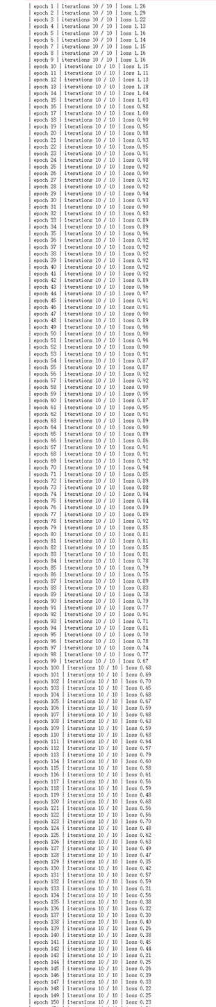
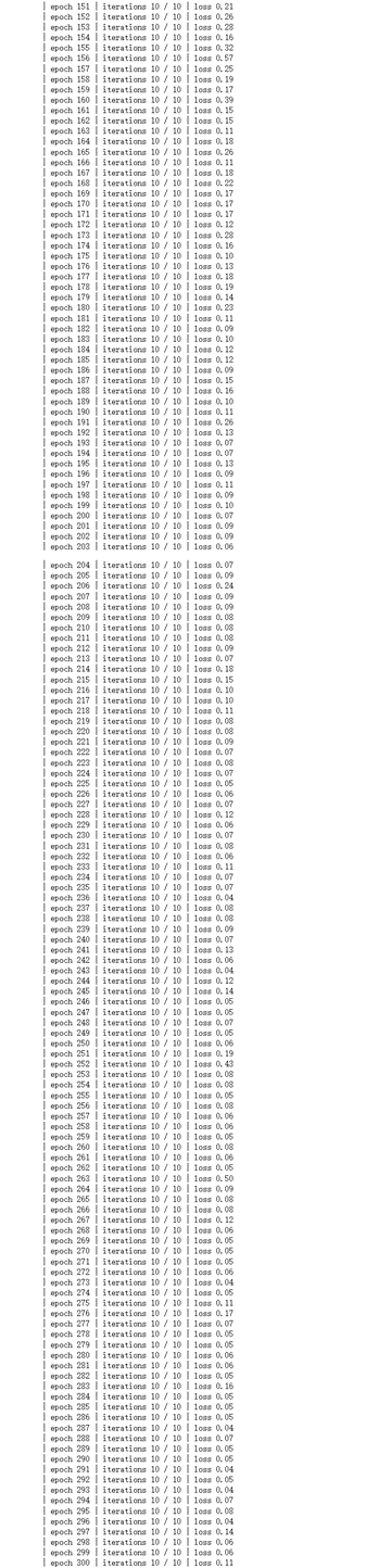
        if (iters+1)%10 == 0:
            avg_loss = total_loss / loss_count
            print('| epoch %d | iterations %d / %d | loss %0.2f'% (epoch+1,iters + 1,max_iters,avg_loss))
            loss_list.append(avg_loss)
            total_loss,loss_count = 0,0

解释：

运行迭代300次的结果图如下：

x, t = load_data()

# 绘制数据点
n = 100
cls_num = 3
markers = ['o', 'x', '^']

# 绘制决策边界
h = 0.001
x_min, x_max = x[:, 0].min() - .1, x[:, 0].max() + .1
y_min, y_max = x[:, 1].min() - .1, x[:, 1].max() + .1
xx, yy = np.meshgrid(np.arange(x_min, x_max, h), np.arange(y_min, y_max, h))
x = np.c_[xx.ravel(), yy.ravel()]
score = model.predict(x)
predict_cls = np.argmax(score, axis=1)
z = predict_cls.reshape(xx.shape)
plt.contourf(xx, yy, z)
for i in range(cls_num):
    plt.scatter(x[i*n:(i+1)*n, 0], x[i*n:(i+1)*n, 1], s=40, marker=markers[i])

plt.axis('off') # 是否关闭坐标轴
plt.show()

解释：

由此产生的图像可以看到相较于两层神经网络的效果更好，三层神经网络的结果如下所示：

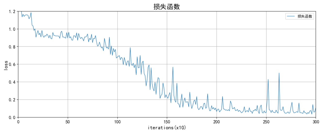
🌻绘制迭代效果图

# loss_list----记录300次迭代次数
import numpy as np
import matplotlib.pyplot as plt
#正确显示中文和负号
plt.rcparams['font.sans-serif']=['simhei']
plt.rcparams['axes.unicode_minus']=false
# 数据准备
x3=range(1,301)
y3=loss_list
# 设置画布大小
plt.figure(figsize=(12, 5))
# plot 画x与y和x与z的关系图
plt.plot(x3,y3,label='损失函数',color='#1f77b4', linewidth=1,marker='',markersize=3)
# 设置x轴标签、坐标轴范围，坐标轴刻度，坐标轴刻度旋转角度
plt.xlabel('iterations(x10)',size=14)
plt.xlim(0,300)
plt.xticks([0,50,100,150,200,250,300],rotation=0,size=12) #
# 设置y轴标签、坐标轴范围，坐标轴刻度，坐标轴刻度旋转角度
plt.ylabel('loss',size=14)
plt.ylim(0,1.2)
plt.yticks([0,0.2,0.4,0.6,0.8,1.0,1.2],rotation=0,size=12)
#标题
plt.title('损失函数',size=18)
# 紧凑布局：自动调整图形、坐标轴、标签之间的距离，对于多个子图时尤其有用。
plt.tight_layout()
# 设置显示图例，要在plt.plot 时设置 label='xxx'才能显示图例
plt.legend()
#加网格线
plt.grid(true)
# 保存图像，可以是任意后缀名，dpi设置图像清晰度
#plt.savefig('./fig1.pdf', dpi=600)  #要放在plt.show()之前，否作保存的图像为空白
# 显示图像
plt.show()

解释：

实验结果如下：

🌞四、实验心得

通过这次实验，我成功创建了一个用于识别螺旋状的数据集三层神经网络，并对深度学习所需的数学知识有了更深入的理解。

一开始，我选择了relu激活函数，但是在调整学习率时无法找到合适的参数。因此改用sigmoid作为激活函数。通过建立三层神经网络，我发现之前适用于两层神经网络的学习率并不适用于三层神经网络，需要重新寻找适合的学习率，而学习率设置得太小会导致学习的收敛速度变慢。

通过对比两层和三层神经网络的训练结果，我发现它们之间存在明显的差异，特别是在中心点区域。这说明增加网络的层数可以更好地拟合复杂的数据集，但也需要仔细调整参数以确保网络的有效训练。

两层神经网络结果：

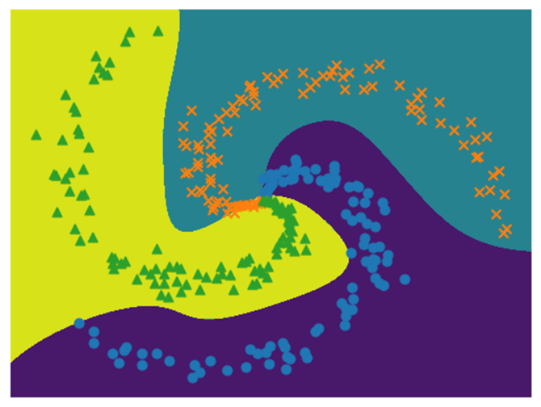
三层神经网络结果：