数据集地址:market basket analysis | kaggle
我的notebook地址:pyspark market basket analysis | kaggle
零售商期望能够利用过去的零售数据在自己的行业中进行探索,并为客户提供有关商品集的建议,这样就能提高客户参与度、改善客户体验并识别客户行为。本文将通过pyspark对数据进行导入与预处理,进行可视化分析并使用spark自带的机器学习库做关联规则学习,挖掘不同商品之间是否存在关联关系。
整体的流程思路借鉴了这个notebook:market basket analysis with apriori🛒 | kaggle
一、导入与数据预处理
这一部分其实没有赘述的必要,贴在这里单纯是为了熟悉pyspark的各个算子。
from pyspark import sparkcontext
from pyspark.sql import functions as f, sparksession, column,types
import pandas as pd
import numpy as np

spark = sparksession.builder.appname("marketbasketanalysis").getorcreate()
data = spark.read.csv("/kaggle/input/market-basket-analysis/assignment-1_data.csv",header=true,sep=";")
data = data.withcolumn("price",f.regexp_replace("price",",",""))
data = data.withcolumn("price",f.col("price").cast("float"))
data = data.withcolumn("quantity",f.col("quantity").cast("int"))
预处理时间类变量
#时间变量
data = data.withcolumn("date_day",f.split("date"," ",0)[0])
data = data.withcolumn("date_time",f.split("date"," ",0)[1])

data = data.withcolumn("hour",f.split("date_time",":")[0])
data = data.withcolumn("minute",f.split("date_time",":")[1])
data = data.withcolumn("year",f.split("date_day","\.")[2])
data = data.withcolumn("month",f.split("date_day","\.")[1])
data = data.withcolumn("day",f.split("date_day","\.")[0])

convert_to_date = f.udf(lambda x:"-".join(x.split(".")[::-1])+" ",types.stringtype())

data = data.withcolumn("date",f.concat(convert_to_date(data["date_day"]),data["date_time"]))
data = data.withcolumn("date",data["date"].cast(types.timestamptype()))

data = data.withcolumn("dayofweek",f.dayofweek(data["date"])-1) #dayofweek这个函数中,以周日为第一天
data = data.withcolumn("dayofweek",f.udf(lambda x:x if x!=0 else 7,types.integertype())(data["dayofweek"]))
删除负值的记录、填充缺失值并删除那些非商品的记录
# 删除price/qty<=0的情况
data = data.filter((f.col("price")>0) & (f.col("quantity")>0))

# 增加total price
data = data.withcolumn("total price",f.col("price")*f.col("quantity"))

data_null_agg = data.agg(
    *[f.count(f.when(f.isnull(c), c)).alias(c) for c in data.columns])
data_null_agg.show()

# customerid 空值填充
data = data.fillna("99999","customerid")

# 删除非商品的那些item
data = data.filter((f.col("itemname")!='postage') & (f.col("itemname")!='dotcom postage') & (f.col("itemname")!='adjust bad debt') & (f.col("itemname")!='manual'))
二、探索性分析
1、总体销售情况
本节开始,将会从订单量(no_of_trans)、成交量(quantity)与成交额(total price)三个维度,分别从多个角度进行数据可视化与分析。
import pandas as pd
from matplotlib import pyplot as plt
import seaborn as sns
from collections import counter

## 总体分析
data_ttl_trans = data.groupby(["billno"]).sum("quantity","total price").withcolumnrenamed("sum(quantity)","quantity").withcolumnrenamed("sum(total price)","total price").topandas()
data_ttl_item = data.groupby(["itemname"]).sum("quantity","total price").withcolumnrenamed("sum(quantity)","quantity").withcolumnrenamed("sum(total price)","total price").topandas()
data_ttl_time = data.groupby(["year","month"]).sum("quantity","total price").withcolumnrenamed("sum(quantity)","quantity").withcolumnrenamed("sum(total price)","total price").topandas()
data_ttl_weekday = data.groupby(["dayofweek"]).sum("quantity","total price").withcolumnrenamed("sum(quantity)","quantity").withcolumnrenamed("sum(total price)","total price").topandas()
data_ttl_country = data.groupby(["country"]).sum("quantity","total price").withcolumnrenamed("sum(quantity)","quantity").withcolumnrenamed("sum(total price)","total price").topandas()
data_ttl_country_time = data.groupby(["country","year","month"]).sum("quantity","total price").withcolumnrenamed("sum(quantity)","quantity").withcolumnrenamed("sum(total price)","total price").topandas()
sns.boxplot(data_ttl_trans["quantity"])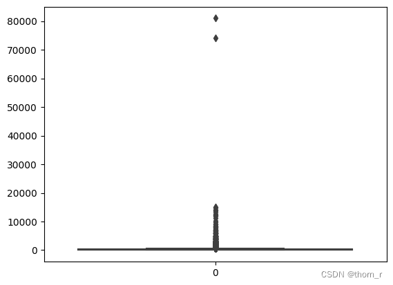
sns.boxplot(data_ttl_trans["total price"])
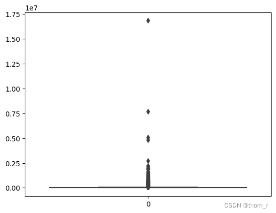
如上两图所示,销售数据极不平衡,有些单子里的销售额或销售量远远超过正常标准,因此在作分布图时,我会将箱线图中的离群点去除。
print("quantity upper",np.percentile(data_ttl_trans["quantity"],75)*2.5-np.percentile(data_ttl_trans["quantity"],25)) #箱线图顶点
print("total price upper",np.percentile(data_ttl_trans["total price"],75)*2.5-np.percentile(data_ttl_trans["total price"],25)) #箱线图顶点
sns.distplot(data_ttl_trans[data_ttl_trans["quantity"]<=661]["quantity"])
sns.distplot(data_ttl_trans[data_ttl_trans["total price"]<=97779]["total price"])
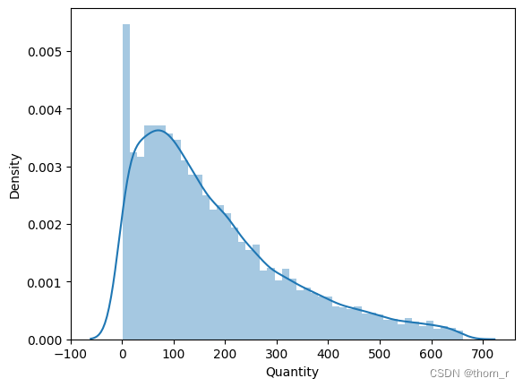
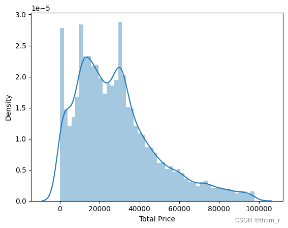
可以看出,哪怕去除了离群点,从分布图上分布看依旧明显右偏趋势,表明了有极少数的订单拥有极大的销售量与销售额,远超正常订单的水平。
sns.boxplot(data_ttl_item["quantity"])
print("quantity upper",np.percentile(data_ttl_item["quantity"],75)*2.5-np.percentile(data_ttl_item["quantity"],25)) #箱线图顶点
#quantity upper 3279.75
sns.distplot(data_ttl_item[data_ttl_item["quantity"]<=2379]["quantity"])

以商品为单位的销量分布也同样右偏,表明了同样有极少数的商品拥有极大的销售量,远超一般商品的水平。
接下来我们看看时间维度上的销量变化
data_ttl_time.index = [str(i)+"\n"+str(j) for i,j in zip(data_ttl_time["year"],data_ttl_time["month"])]
fig,ax1 = plt.subplots()
ax1.plot(data_ttl_time["quantity"],color='gray',label="quantity")
ax2 = ax1.twinx()
ax2.plot(data_ttl_time["total price"],color="red",label="total price")
ax1.set_ylabel("quantity",color="gray")
ax2.set_ylabel("total price",color="red")
plt.show()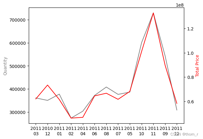
plt.bar(data_ttl_weekday["dayofweek"],data_ttl_weekday["total price"],color='red',width=0.5,label="quantity")
plt.show() #周六不卖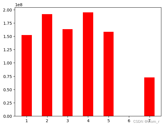
从时间轴上来看,销售额有一个明显的上升趋势,到了11月有一个明显的高峰,而到12月则有所回滚。
data_ttl_country.index = data_ttl_country["country"]
ttl_price_country = data_ttl_country["total price"].sort_values()[::-1]
tmp = ttl_price_country[5:]
ttl_price_country = ttl_price_country[0:5]
ttl_price_country["others"] = sum(tmp)
plt.pie(ttl_price_country,labels=ttl_price_country.index)
plt.legend(loc="upper right")
plt.show()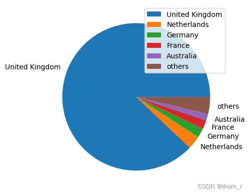
data_ttl_country_time["isunitedkingdom"]=["uk" if i=="united kingdom" else "not uk" for i in data_ttl_country_time["country"]]
data_ttl_country_time_isuk = data_ttl_country_time.groupby(["isunitedkingdom","year","month"])["total price"].sum().reset_index()
data_ttl_country_time_isuk.index = data_ttl_country_time_isuk["year"]+"\n"+data_ttl_country_time_isuk["month"]
uk = data_ttl_country_time_isuk[data_ttl_country_time_isuk["isunitedkingdom"]=="uk"]
nuk = data_ttl_country_time_isuk[data_ttl_country_time_isuk["isunitedkingdom"]=="not uk"]
plt.figure(figsize=(8,8))
plt.bar(uk.index,uk["total price"],color="#66c2a5",label="united kingdom")
plt.bar(nuk.index,nuk["total price"],bottom=uk["total price"],color="#8da0cb",label="other country")
plt.legend()
plt.show()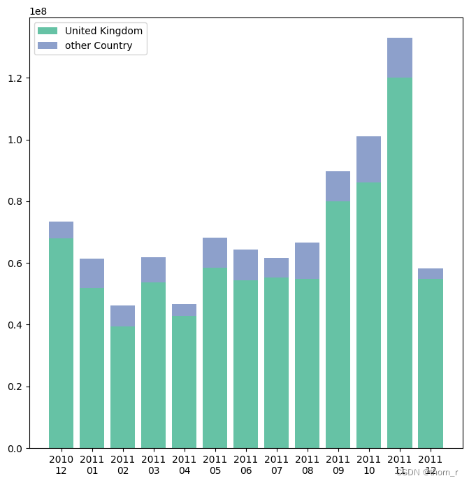
总体上来看,总销售额的绝大部分都是来自于英国销售,而从时间线商来看,每个月都是英国销售额占主体。因此,后文的分析将看2011年英国的全年销售。
## 只选取uk2011年的全年数据
df_uk = data.filter((f.col("country")=="united kingdom") & (f.col("year")==2011))
2、是否存在季节性商品
首先,我们将2011年的4个季度的销售额、销售量以及成交量分别汇总并排序,看看有没有哪个商品在各个季度的排名有明显的差距。
def transform_to_season(x):
    if len(x)>1 and x[0]=="0":
        x = x[1:]
    return int((int(x)-1)//3)+1

df_uk = df_uk.withcolumn("season",f.udf(transform_to_season,types.integertype())(f.col("month")))

df_uk_seasonal = df_uk.groupby(["season","itemname"]).agg(f.countdistinct(f.col("billno")).alias("no_of_trans"),f.sum(f.col("quantity")).alias("quantity")
                                                         ,f.sum(f.col("total price")).alias("total price")).topandas()

# 排序
def rank_seasonal(df,season="all"):
    groupby_cols = ["itemname"]
    if season!="all":
        groupby_cols.append("season")
        df = df[df["season"]==int(season)]
    df = df.groupby(groupby_cols).sum(["no_of_trans","quantity","total price"])
    for col in ["no_of_trans","quantity","total price"]:
        df[col+"_rank"]=df[col].rank(ascending=false)
    return df

df_uk_all = rank_seasonal(df_uk_seasonal)
df_uk_first = rank_seasonal(df_uk_seasonal,"1")
df_uk_second = rank_seasonal(df_uk_seasonal,"2")
df_uk_third = rank_seasonal(df_uk_seasonal,"3")
df_uk_fourth = rank_seasonal(df_uk_seasonal,"4")

## top 10 rank:
dfs = [df_uk_all,df_uk_first,df_uk_second,df_uk_third,df_uk_fourth]
item_set_no_of_trans=set()
item_set_quantity=set()
item_set_total_price = set()
for df in dfs:
    df = df.copy().reset_index()
    itemname_top_trans = df[df["no_of_trans_rank"]<=10]["itemname"]
    itemname_top_qty = df[df["quantity_rank"]<=10]["itemname"]
    itemname_top_ttl_price = df[df["total price_rank"]<=10]["itemname"]
    for i in itemname_top_trans:
        item_set_no_of_trans.add(i)
    for i in itemname_top_qty:
        item_set_quantity.add(i)
    for i in itemname_top_ttl_price:
        item_set_total_price.add(i)

## 每个季度的是否有所不同?
rank_df = {"dimension":[],"item":[],"rank":[],"value":[],"season":[],"range":[]}#pd.dataframe(columns=["dimension","item","rank","value"])

for dim,itemset in [("no_of_trans",item_set_no_of_trans),("quantity",item_set_quantity),("total price",item_set_total_price)]:
    for i in list(itemset):
        min_rank=9999
        max_rank=-1
        for j,df in enumerate(dfs):
            df = df.reset_index()
            if j == 0:
                rank_df["season"].append("all")
            else:
                rank_df["season"].append(df["season"].values[0])
            sub_df = df[df["itemname"]==i]
            if sub_df.shape[0]==0:
                curr_rank=9999
                curr_value=0
            else:
                curr_rank = df[df["itemname"]==i][dim+"_rank"].values[0]
                curr_value = df[df["itemname"]==i][dim].values[0]
            min_rank = min(curr_rank,min_rank)
            max_rank = max(curr_rank,max_rank) if curr_rank<9999 else max_rank
            rank_df["dimension"].append(dim)
            rank_df["item"].append(i)
            rank_df["rank"].append(curr_rank)
            rank_df["value"].append(curr_value)
        rank_df["range"] += [max_rank-min_rank]*5
rank_df = pd.dataframe(rank_df)

plt.figure(figsize=(20,20))
# “每个季度的量相差很多”的,但是本身很多的
dims = ["no_of_trans","quantity","total price"]
for i,dim in enumerate(dims):
    tmp_df = rank_df[(rank_df["dimension"]==dim) & (rank_df["season"]!='all')]
    tmp_df["range_rank"] = tmp_df["range"].rank(ascending=false)
    tmp_df = tmp_df.sort_values("range_rank").reset_index(drop=true)
    for j in range(3):
        tmp_df_rank = tmp_df.loc[4*j:4*(j+1)-1,:]
        this_item = list(set(tmp_df_rank["item"]))[0]
        plt.subplot(3,3,i*3+j+1)
        plt.pie(tmp_df_rank["value"],labels=tmp_df_rank["season"])
        plt.title(f"{dim}:{this_item}")
plt.show()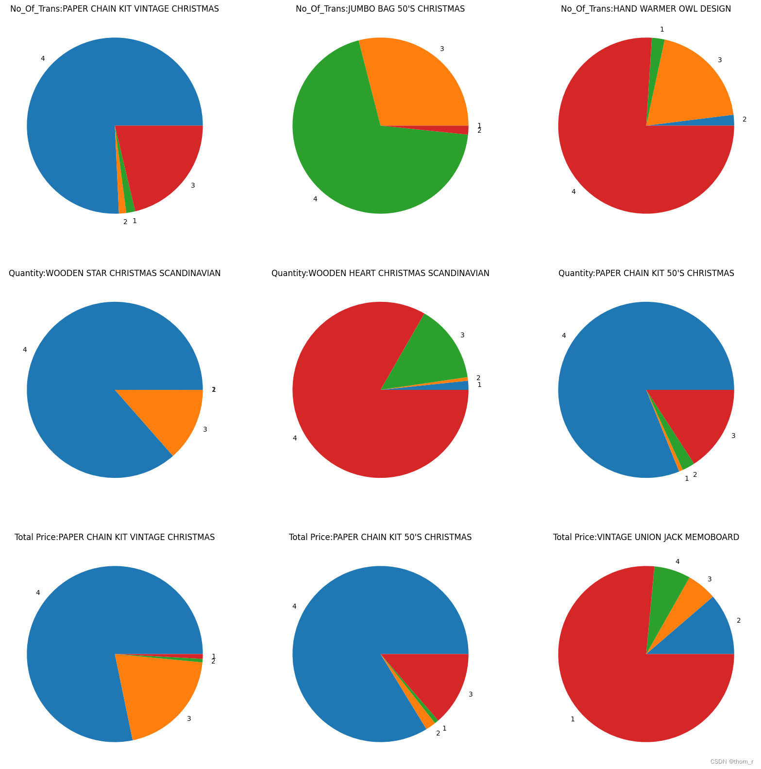
上图中的商品,是在全年的销售中名销售额/销售了/成交量列前茅的几个商品,但是从饼图上来看,这下商品明显是会集中在某一个季度中畅销。我们把颗粒度缩小到按月份来看,计算每月销售额占总销售额的比重(季节指数);并以此排序看看哪些商品的季节指数极差最大。
df_uk_monthly = df_uk.groupby(["month","itemname"]).agg(f.countdistinct(f.col("billno")).alias("no_of_trans"),f.sum(f.col("quantity")).alias("quantity")
                                                         ,f.sum(f.col("total price")).alias("total price")).topandas().reset_index(drop=true)

df_uk_fullyear = df_uk_monthly.groupby(["itemname"]).mean(["no_of_trans","quantity","total price"]).reset_index()
df_uk_fullyear.rename(columns={"no_of_trans":"fy_no_of_trans","quantity":"fy_quantity","total price":"fy_total price"},inplace=true)

df_uk_monthly_season = pd.merge(df_uk_monthly,df_uk_fullyear,on=["itemname"],how='left')
df_uk_monthly_season["seasonal_index_no_of_trans"]=df_uk_monthly_season["no_of_trans"]/df_uk_monthly_season["fy_no_of_trans"]
df_uk_monthly_season["seasonal_index_quantity"]=df_uk_monthly_season["quantity"]/df_uk_monthly_season["fy_quantity"]
df_uk_monthly_season["seasonal_index_total price"]=df_uk_monthly_season["total price"]/df_uk_monthly_season["fy_total price"]

#算极差

df_uk_season_max = df_uk_monthly_season.groupby("itemname").max(["seasonal_index_no_of_trans","seasonal_index_quantity","seasonal_index_total price"]).reset_index().rename(columns={"seasonal_index_no_of_trans":"seasonal_index_no_of_trans_max","seasonal_index_quantity":"seasonal_index_quantity_max","seasonal_index_total price":"seasonal_index_total price_max"})
df_uk_season_min = df_uk_monthly_season.groupby("itemname").min(["seasonal_index_no_of_trans","seasonal_index_quantity","seasonal_index_total price"]).reset_index().rename(columns={"seasonal_index_no_of_trans":"seasonal_index_no_of_trans_min","seasonal_index_quantity":"seasonal_index_quantity_min","seasonal_index_total price":"seasonal_index_total price_min"})
df_uk_season_ranges = pd.merge(df_uk_season_min,df_uk_season_max,on=["itemname"])
seasonal_index_cols = ["seasonal_index_no_of_trans","seasonal_index_quantity","seasonal_index_total price"]
for col in seasonal_index_cols:
    df_uk_season_ranges[col] = df_uk_season_ranges[col+"_max"]-df_uk_season_ranges[col+"_min"]
    df_uk_season_ranges[col+"_rank"]=df_uk_season_ranges[col].rank(ascending=false)
df_uk_season_ranges = df_uk_season_ranges[["itemname"]+[i for i in df_uk_season_ranges if "seasonal_index" in i]]

plt.figure(figsize=(15,15))
for i,col in enumerate(["seasonal_index_no_of_trans","seasonal_index_quantity","seasonal_index_total price"]):
    seasonal_items = df_uk_season_ranges.sort_values(col+"_rank").reset_index().loc[:2,"itemname"].tolist()
    for j,item in enumerate(seasonal_items):
        plt.subplot(3,3,i*3+j+1)
        idxs = [k for k in df_uk_monthly.index if df_uk_monthly.loc[k,"itemname"]==item]
        tmp_df = df_uk_monthly.loc[idxs,["itemname","month",col.replace("seasonal_index_","")]]
        tmp_df = tmp_df.pivot(index="month",columns="itemname",values=col.replace("seasonal_index_",""))
        plt.plot(tmp_df, marker='o')
        plt.ylabel(col.replace("seasonal_index_",""))
        plt.title(item)

plt.show()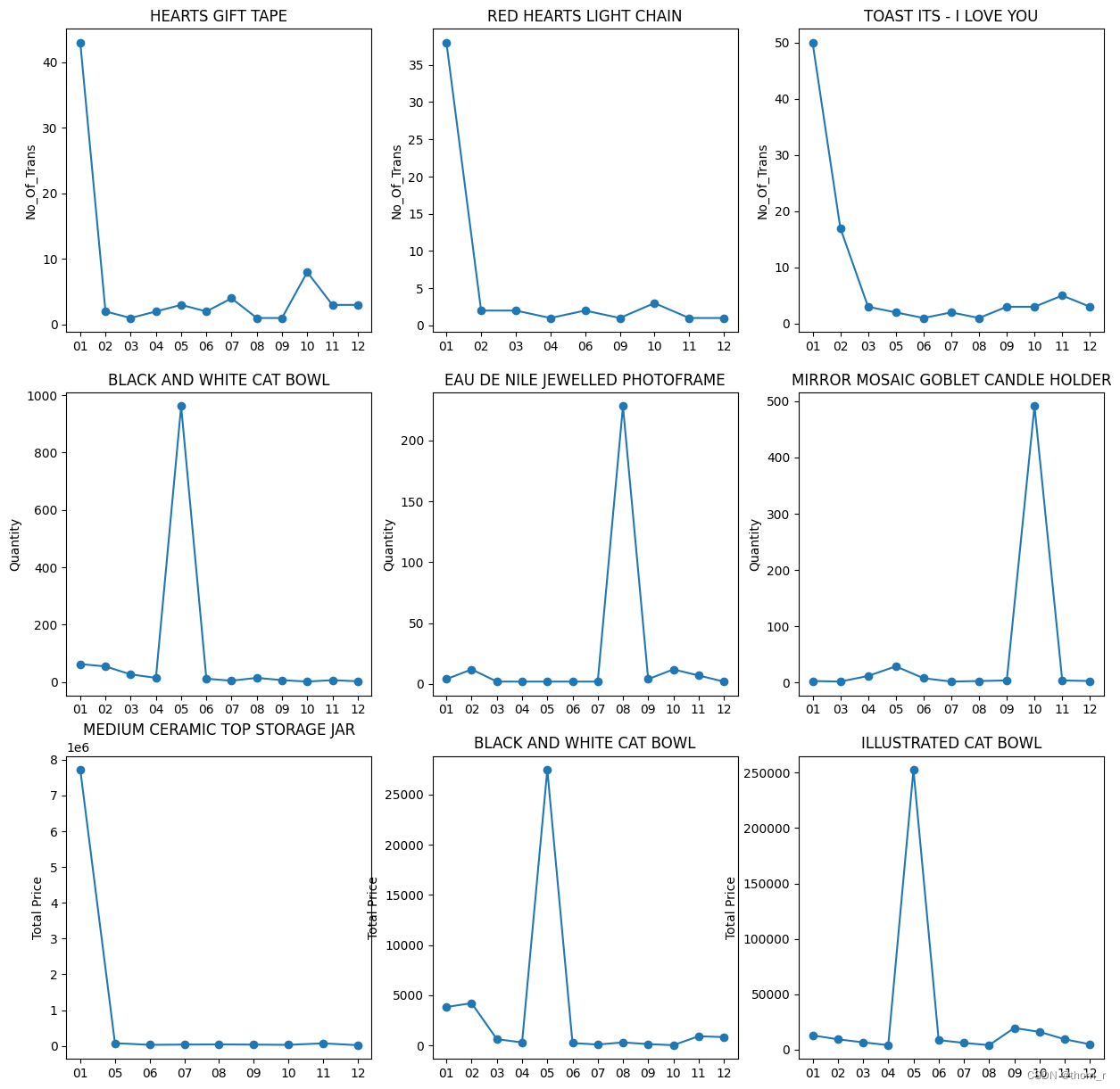
此处分别从销售额/销售量/成交量3个维度构造了季节指数,并将极差排名前3的商品作了折线统计图。从途中来看,这些商品全都是“集中在某一个月份十分畅销,但是在其他月份相对无人问津”。
ranges = rank_df.groupby(["dimension","item"]).first(["range"]).reset_index()[["dimension","item","range"]]

## no_of_trans
plt.figure(figsize=(20,20))
range_df = ranges[ranges["dimension"]=="no_of_trans"]
titles = ["all","season one","season two","season three","season four"]
for n in range(5):
    plt.subplot(5,1,n+1)
    df = dfs[n].copy().reset_index()
    df = df.loc[[i for i in df.index if df.loc[i,"itemname"] in item_set_no_of_trans],["itemname","no_of_trans"]]
    df=df.sort_values("no_of_trans",ascending=false)
    df = df.iloc[:10,:]
    df = pd.merge(df,range_df,left_on="itemname",right_on="item",how="left")
    plt.barh(df["itemname"]+" "+df["range"].astype("str"),df["no_of_trans"])
    plt.title("no_of_trans "+titles[n])
plt.show()

plt.figure(figsize=(20,20))
range_df = ranges[ranges["dimension"]=="quantity"]
titles = ["all","season one","season two","season three","season four"]
for n in range(5):
    plt.subplot(5,1,n+1)
    df = dfs[n].copy().reset_index()
    df = df.loc[[i for i in df.index if df.loc[i,"itemname"] in item_set_quantity],["itemname","quantity"]]
    df=df.sort_values("quantity",ascending=false)
    df = df.iloc[:10,:]
    df = pd.merge(df,range_df,left_on="itemname",right_on="item",how="left")
    plt.barh(df["itemname"]+" "+df["range"].astype("str"),df["quantity"])
    plt.title("quantity "+titles[n])
plt.show()

plt.figure(figsize=(20,20))
range_df = ranges[ranges["dimension"]=="total price"]
titles = ["all","season one","season two","season three","season four"]
for n in range(5):
    plt.subplot(5,1,n+1)
    df = dfs[n].copy().reset_index()
    df = df.loc[[i for i in df.index if df.loc[i,"itemname"] in item_set_total_price],["itemname","total price"]]
    df=df.sort_values("total price",ascending=false)
    df = df.iloc[:10,:]
    df = pd.merge(df,range_df,left_on="itemname",right_on="item",how="left")
    plt.barh(df["itemname"]+" "+df["range"].astype("str"),df["total price"])
    plt.title("total price "+titles[n])
plt.show()
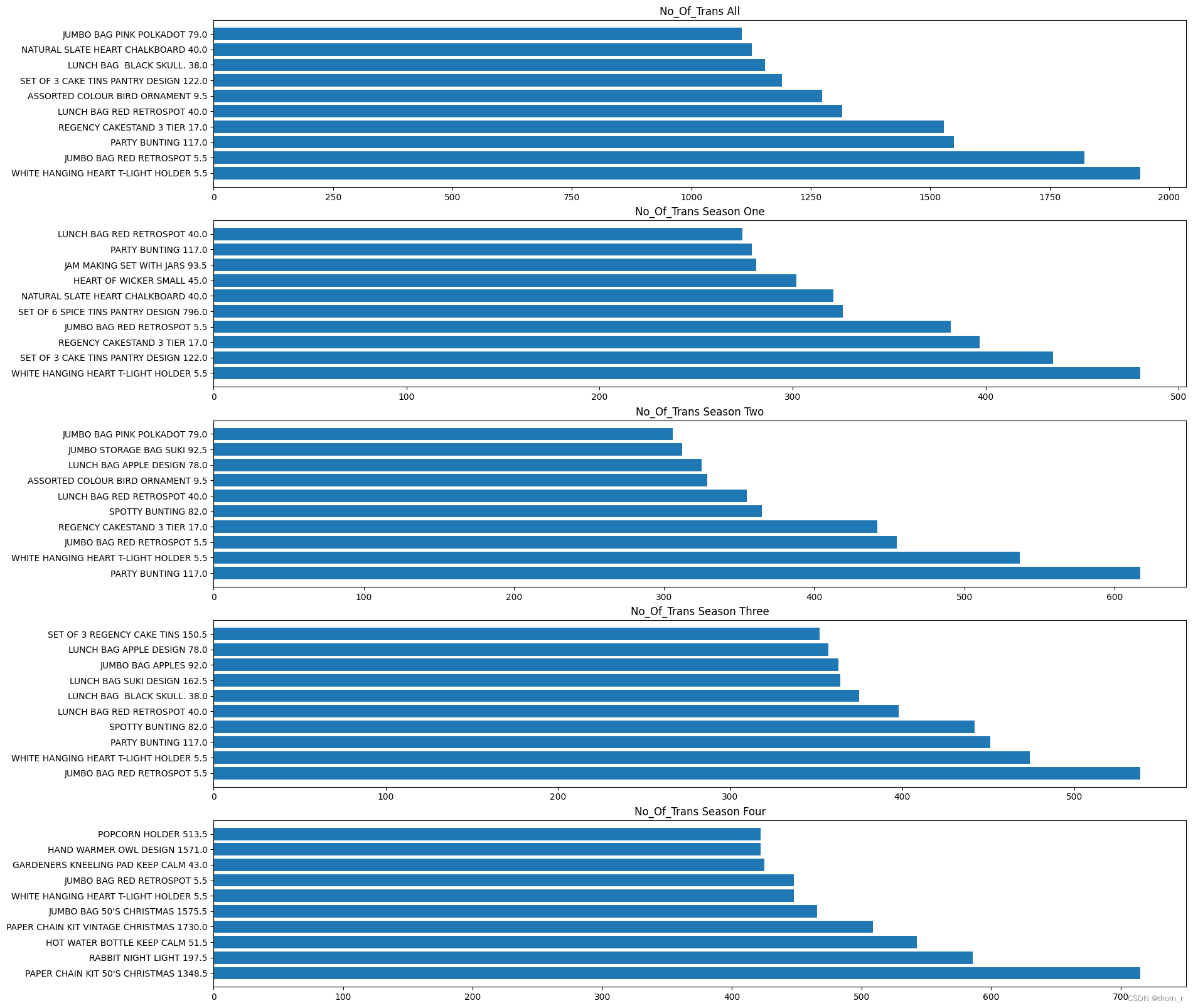
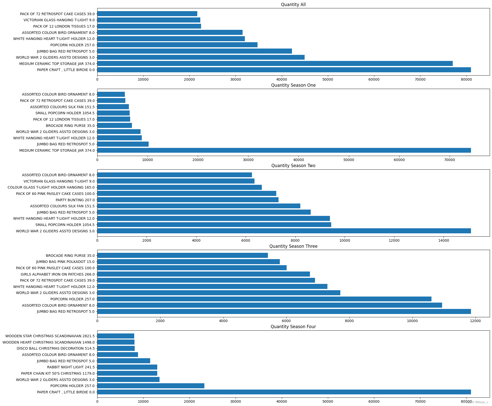
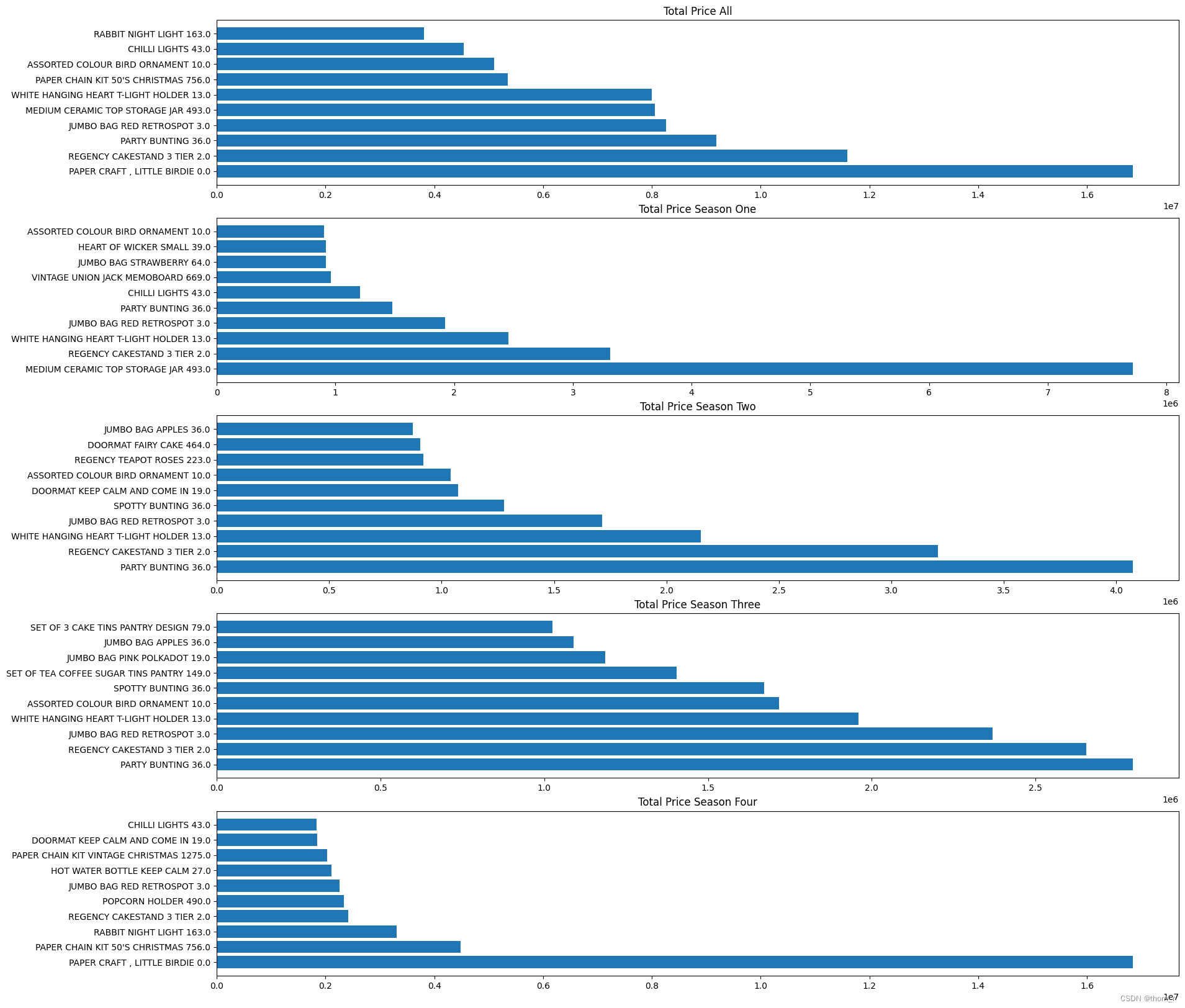
最终将全年的top10以及每个季度的top10作图,图中商品旁边标出了它对应销售额/销售量/成交量的排名的极差,可以看到,虽然大多数在全年销售中获得的top10排名极差都较小(总共有3000+个商品),但是在总销售额的全年top10中,依然有一个明显存在季节性效应的商品(paper chain kit 50's chrismas)。
3、同一个商品在不同维度上是否排名差距较大
df_uk_all = df_uk_monthly.groupby(["itemname"]).sum(["no_of_trans","quantity","total price"]).reset_index()
df_uk_all["no_of_trans_rank"] = df_uk_all["no_of_trans"].rank(ascending=false)
df_uk_all["quantity_rank"] = df_uk_all["quantity"].rank(ascending=false)
df_uk_all["total price_rank"] = df_uk_all["total price"].rank(ascending=false)

rank_gaps = [max(df_uk_all.loc[i,"no_of_trans_rank"],df_uk_all.loc[i,"quantity_rank"],df_uk_all.loc[i,"total price_rank"])\
             - min(df_uk_all.loc[i,"no_of_trans_rank"],df_uk_all.loc[i,"quantity_rank"],df_uk_all.loc[i,"total price_rank"])\
             for i in range(df_uk_all.shape[0])]
df_uk_all["rank_gaps"] = rank_gaps

df_ranked_all = df_uk_all.sort_values("rank_gaps",ascending=false).reset_index(drop=true)

plt.figure(figsize=(20,20))
for i in range(5):
    plt.subplot(5,1,i+1)
    sub = df_ranked_all.iloc[i,:]
    item_name = sub["itemname"]
    sub = dict(sub)
    sub_df = pd.dataframe({"index":["no_of_trans_rank","quantity_rank","total price_rank"],\
                           "value":[sub["no_of_trans_rank"],sub["quantity_rank"],sub["total price_rank"]]})
    plt.barh(sub_df["index"],sub_df["value"])
    plt.title(item_name)
plt.show()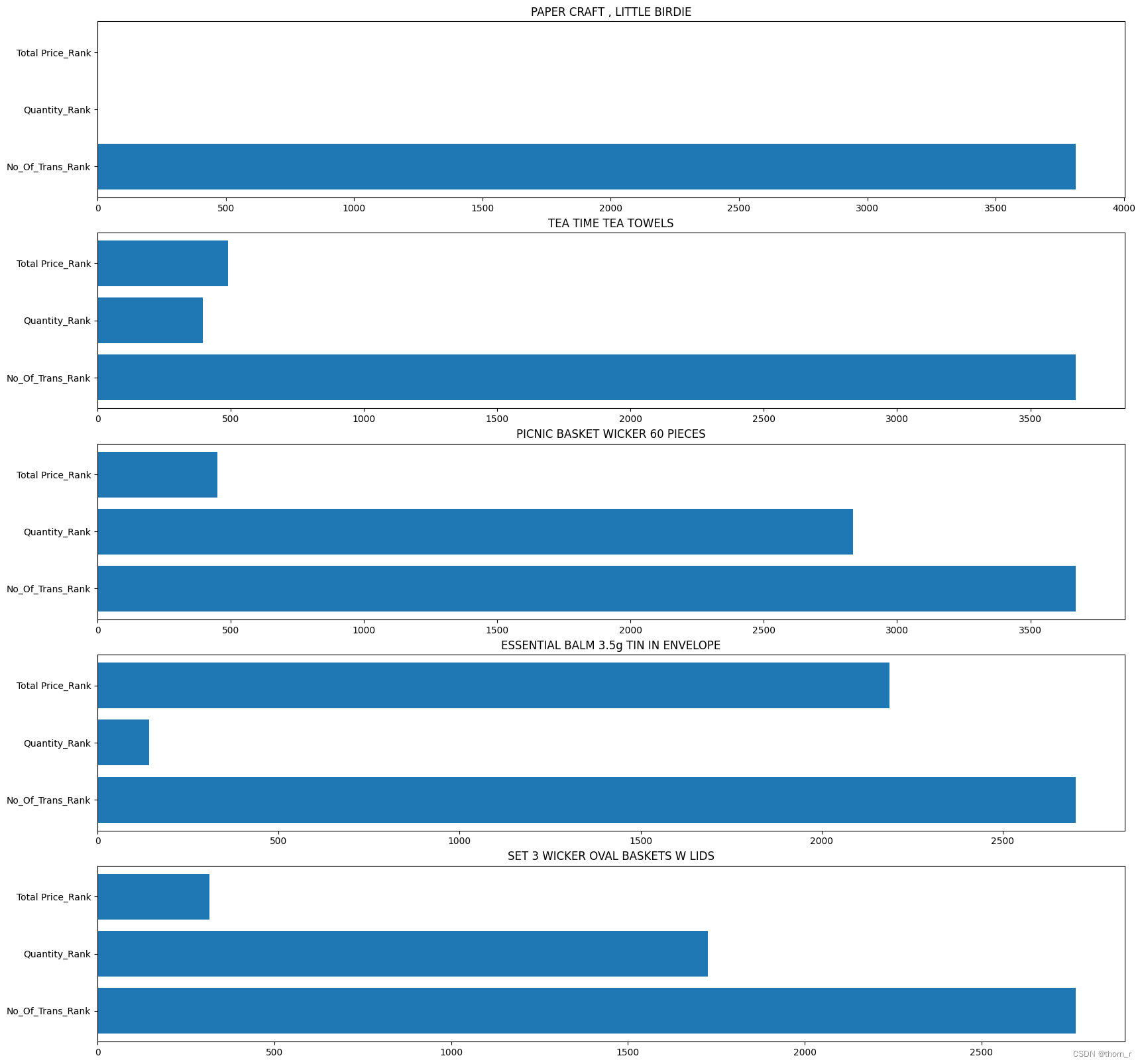
这里计算了每件商品在销售额、销售量、成交量上的排名并将这三个排名相差最大的5个商品列出了。可以发现上图中的商品,有些虽然销售额与销售量名列前茅,但是成交量却排名靠后。特别是第一名(paper craft, little bride),实际看表格数据时会发现它只有1个单子,但是那1个单子却订了8万多个这个商品。
4、探索客单价、客单量与平均售价
现在构造以下3个kpi:
客单量(upt)= 销售量(quantity)/成交量(no_of_trans)
平均售价(asp)= 销售额(total price)/ 销售量(quantity)
客单价(atv)= 销售额(total price)/ 成交量(no_of_trans)
df_uk_monthly_kpi = df_uk_monthly.groupby(["month"]).sum(["no_of_trans","quantity","total price"]).reset_index()
df_uk_monthly_kpi["upt"] = df_uk_monthly_kpi["quantity"]/df_uk_monthly_kpi["no_of_trans"]
df_uk_monthly_kpi["atv"] = df_uk_monthly_kpi["total price"]/df_uk_monthly_kpi["no_of_trans"]
df_uk_monthly_kpi["asp"] = df_uk_monthly_kpi["total price"]/df_uk_monthly_kpi["quantity"]

plt.plot(df_uk_monthly_kpi["month"],df_uk_monthly_kpi["upt"])
plt.title("unit per transaction")
plt.show()
plt.plot(df_uk_monthly_kpi["month"],df_uk_monthly_kpi["atv"])
plt.title("average transaction value")
plt.show()
plt.plot(df_uk_monthly_kpi["month"],df_uk_monthly_kpi["asp"])
plt.title("average selling price")
plt.show()

plt.plot(df_uk_monthly_kpi["month"],df_uk_monthly_kpi["no_of_trans"])
plt.title("no_of_trans")
plt.show()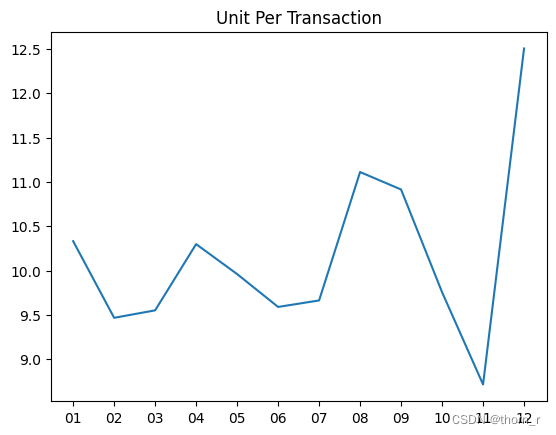

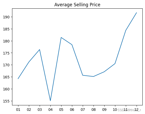
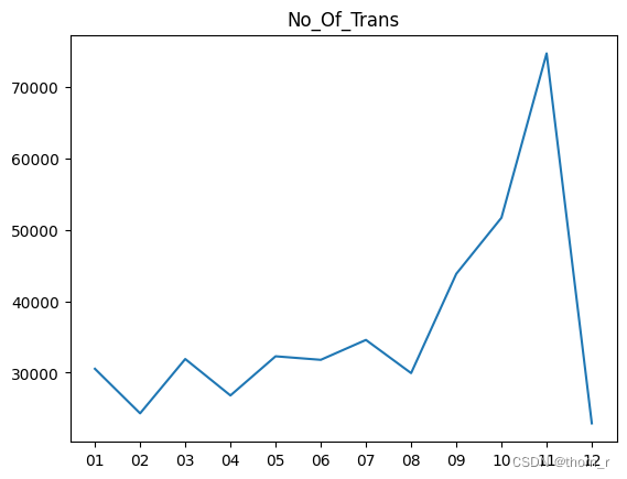
这里可以得出一个非常有趣的结论。11月的高销售额实际上是由于11月的高交易量。尽管12月份的销售额再次下降,但12月份的订单大多都是大单子。
5、(待定)探索客户价值
此处把customer id不为空的数据当做是会员数据
df_monthly_customerid = df_uk.groupby(["customerid","month"]).agg(f.countdistinct(f.col("billno")).alias("no_of_trans"),f.sum(f.col("quantity")).alias("quantity")
                                                        ,f.sum(f.col("total price")).alias("total price")).topandas()
df_by_customerid_by_item = df_uk.groupby(["customerid","itemname"]).agg(f.countdistinct(f.col("billno")).alias("no_of_trans"),f.sum(f.col("quantity")).alias("quantity")
                                                        ,f.sum(f.col("total price")).alias("total price")).topandas()

df_monthly_customerid["customerid"] = df_monthly_customerid["customerid"].astype(str)
df_monthly_customerid["ismember"] = [str(i)!='99999' for i in df_monthly_customerid["customerid"]]

df_monthly_member = df_monthly_customerid[df_monthly_customerid["ismember"]==true].groupby("month").sum(["no_of_trans","total price"]).sort_index()
df_monthly_non_member = df_monthly_customerid[df_monthly_customerid["ismember"]==false].reset_index()
df_monthly_non_member.index=df_monthly_non_member["month"]
df_monthly_non_member = df_monthly_non_member.sort_index()

plt.figure(figsize=(8,8))
plt.bar(df_monthly_member.index,df_monthly_member["total price"],color="#66c2a5",label="member")
plt.bar(df_monthly_non_member.index,df_monthly_non_member["total price"],bottom=df_monthly_member["total price"],color="#8da0cb",label="non-member")
plt.legend()
plt.show()

df_monthly_member_no_of_trans = df_monthly_customerid[df_monthly_customerid["ismember"]==true].groupby("month").sum("no_of_trans").sort_index()
plt.figure(figsize=(8,8))
plt.bar(df_monthly_member_no_of_trans.index,df_monthly_member_no_of_trans["no_of_trans"],color="#66c2a5",label="member")
plt.bar(df_monthly_non_member.index,df_monthly_non_member["no_of_trans"],bottom=df_monthly_member_no_of_trans["no_of_trans"],color="#8da0cb",label="non-member")
plt.legend()
plt.show()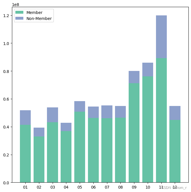
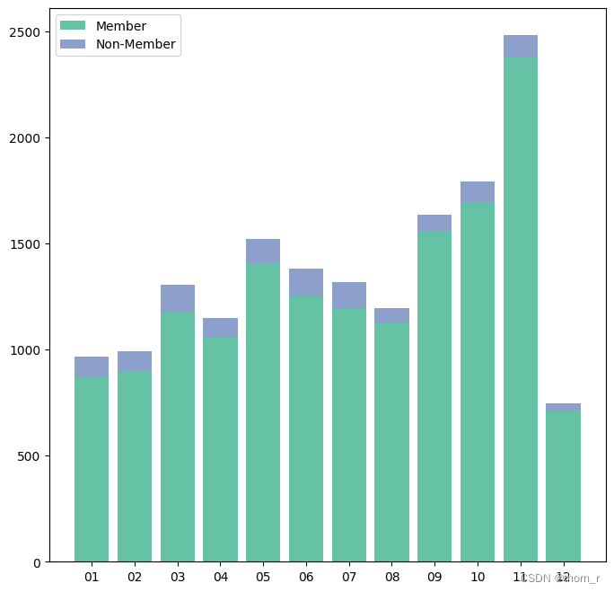
从图中来看,无论是交易量还是销售额,都是会员销售占大多数的。这样的结论对我而言过于反直觉,因此我没有做后续的分析。
三、关联规则分析
关联规则分析为的就是发现商品与商品之间的关联。通过计算商品之间的支持度、置信度与提升度,分析哪些商品有正向关系,顾客愿意同时购买它们。
此处使用了pyspark自带的fpgrowth算法。它和apriori算法一样都是计算两两商品之间支持度置信度与提升度的算法,虽然算法流程不同,但是计算结果是一样的。
from pyspark.ml.fpm import fpgrowth,fpgrowthmodel
df_uk_concatenated=df_uk.groupby(["billno","itemname"]).agg(f.sum("quantity").alias("quantity")).groupby("billno").agg(f.collect_list(f.col("itemname")).alias("items"))

model = fpgrowth(minsupport=0.03,minconfidence=0.3)
model = model.fit(df_uk_concatenated.select("items"))

res = model.associationrules.topandas()
import itertools

combs = [('confidence', 'lift', 'support'),('lift', 'support', 'confidence'),('support', 'confidence', 'lift')]

for i,(x,y,c) in enumerate(combs):
    plt.subplot(3,1,i+1)
    sc = plt.scatter(res[x],res[y],c=res[c],cmap='viridis')
    plt.xlabel(x)
    plt.ylabel(y)
    plt.colorbar(sc,label=c)
plt.show()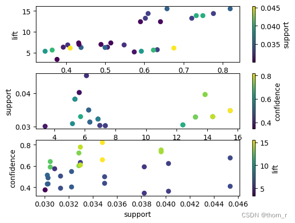
res.sort_values("support",ascending=false).head(6)
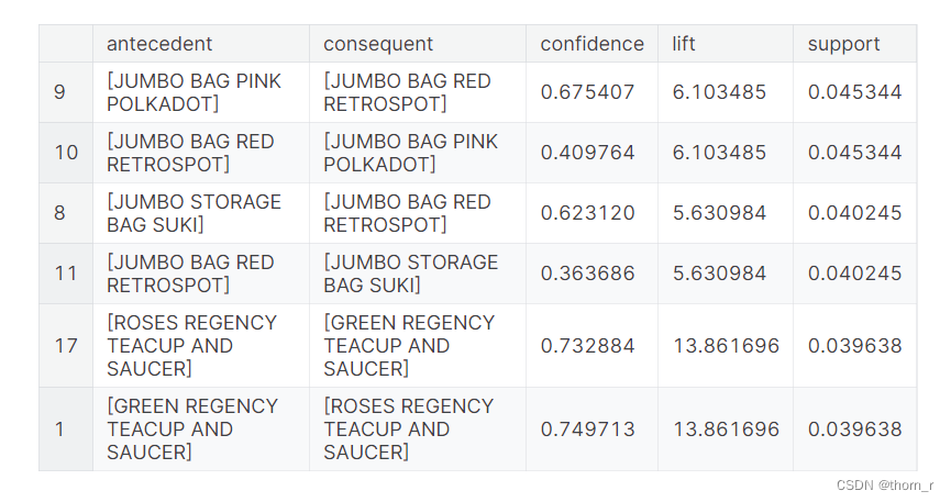
上图是支持度(support)前三的商品组合(每2条实际上是同一组商品)。
支持度指的是2件商品同时出现的概率。
res.sort_values("confidence",ascending=false).head(5)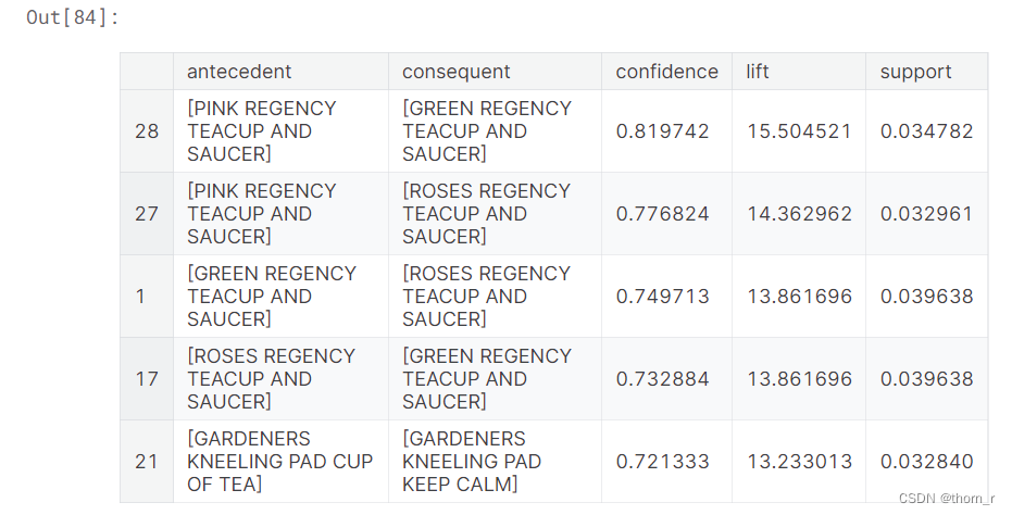
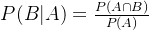
上图是置信度(confidence)前5的商品组合,置信度指的是当商品a被购买时,商品b也被购买的概率。
res.sort_values("lift",ascending=false).head(6)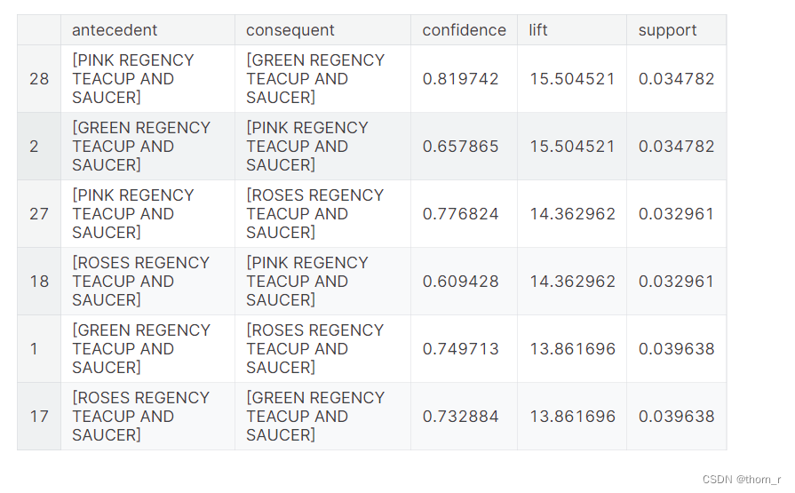
上图是提升度(lift)前三的商品组合(每2条实际上是同一组商品)。 提升度可以看做是2件商品之间是否存在正向/反向的关系。
最后将提升度降序排列打印出来:
res.sort_values("lift",ascending=false)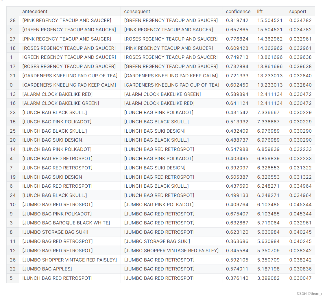
我们发现顾客最常见的组合是不同颜色的杯子和碟子。
其他产品,如午餐袋、jumbo bag或闹钟也处于同样的情况。
总的来说,最常见的组合是同一种产品不同的颜色。
四、结论
1、英国2011年时11月份销售量急剧上升,12月份又有所回落
2、11月的销售量高是因为11月的成交量大,而在12月,虽然销售量相对较小,但实际上12月的每笔交易都是大交易,数量和价格都很大。
3、许多产品都有季节性影响,即使是当年销量排名前10的产品(paper chain kit 50’s chrismas)
4、有些产品虽然交易量很少,但销量却遥遥领先(如paper craft, little birdie, 2011年只有1笔交易,但销量第一)。
5、最常见的组合是同一产品不同颜色的组合。最典型的例子就是杯子和碟子。


发表评论