前言
生成式建模的扩散思想实际上已经在2015年(sohl-dickstein等人)提出,然而,直到2019年斯坦福大学(song等人)、2020年google brain(ho等人)才改进了这个方法,从此引发了生成式模型的新潮流。目前,包括openai的glide和dall-e 2,海德堡大学的latent diffusion和google brain的imagegen,都基于diffusion模型,并可以得到高质量的生成效果。本文以下讲解主要基于ddpm,并适当地增加一些目前有效的改进内容。
基本原理
扩散模型包括两个步骤:
固定的(或预设的)前向扩散过程q:该过程会逐渐将高斯噪声添加到图像中,直到最终得到纯噪声。
可训练的反向去噪扩散过程
 :训练一个神经网络,从纯噪音开始逐渐去噪,直到得到一个真实图像。
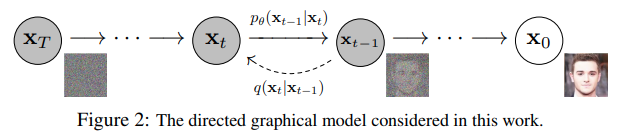
前向与后向的步数由下标 t定义,并且有预先定义好的总步数 t(ddpm原文中为1000)。
t=0 时为从数据集中采样得到的一张真实图片, t=t 时近似为一张纯粹的噪声。
2.1 直观理解
2.2 数学形式
2.2.1 前向过程
 是真实数据分布(也就是真实的大量图片),从这个分布中采样即可得到一张真实图片
  。我们定义前向扩散过程为
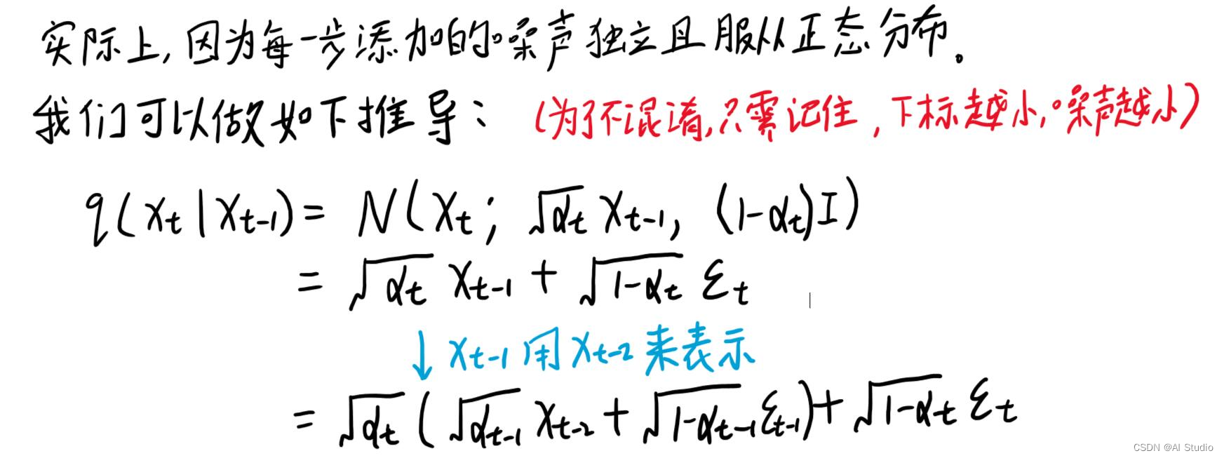
  ,即每一个step向图片添加噪声的过程,并定义好一系列
 ,则有:
,则有:
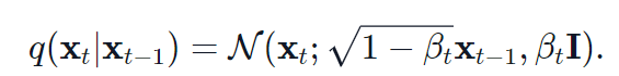
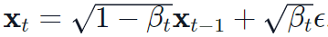
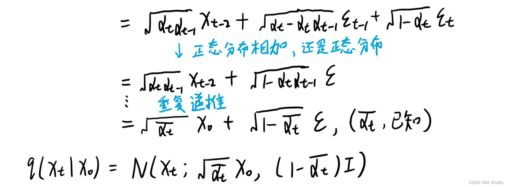
其中,n为正态分布,均值和方差分别为 ,因此通过采样标准正态分布
 ,有:
,有:
2.2.2 反向过程
那么问题的核心就是如何得到的逆过程 ,这个过程无法直接求出来,所以我们使用神经网络去拟合这一分布。我们使用一个具有参数的神经网络去计算
  。假设反向的条件概率分布也是高斯分布,且高斯分布实际上只有两个参数:均值和方差,那么神经网络需要计算的实际上是

在ddpm中,方差被固定,网络只学习均值。而之后的改进模型中,方差也可由网络学习得到。

2.2.3 总结过程
2.3 网络训练流程
我们最终要训练的实际上是一个噪声预测器。神经网络输出的噪声是 ,而真实的噪声取自于正态分布。则损失函数为:

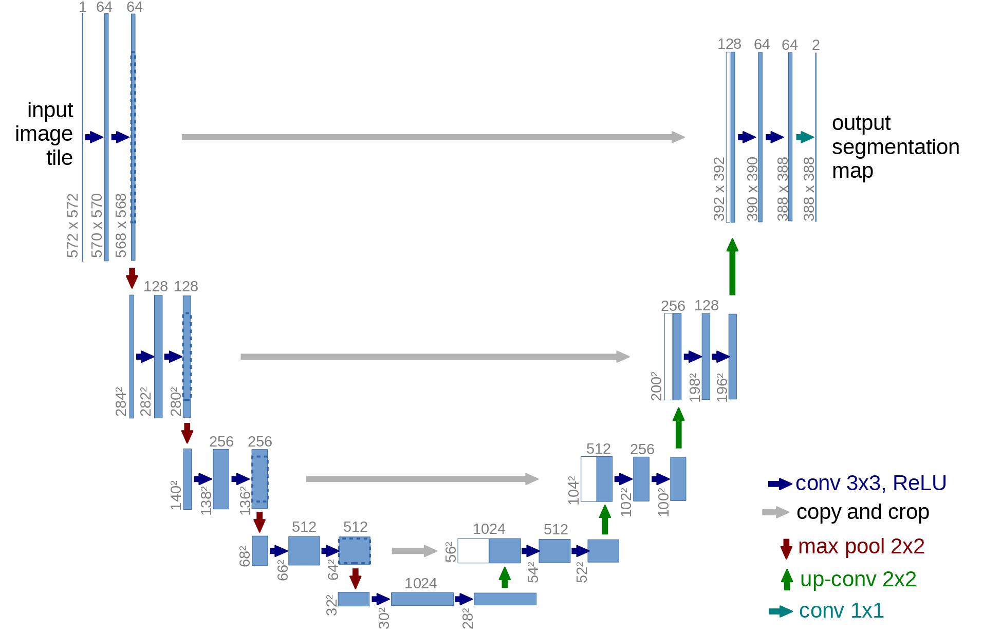
预测网络方面,ddpm采用了 u-net。
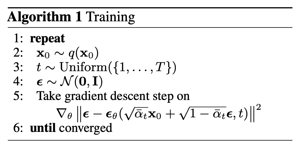
从而,网络的训练流程为:
我们接受一个随机的样本
;
我们随机从 1 到 t 采样一个 t;
我们从高斯分布采样一些噪声并且施加在输入上;
网络从被影响过后的噪声图片学习其被施加了的噪声。
代码
3.1 network helpers
先是一些辅助函数和类。
def exists(x):
    return x is not none

# 有val时返回val,val为none时返回d
def default(val, d):
    if exists(val):
        return val
    return d() if isfunction(d) else d

# 残差模块,将输入加到输出上
class residual(nn.module):
    def __init__(self, fn):
        super().__init__()
        self.fn = fn

    def forward(self, x, *args, **kwargs):
        return self.fn(x, *args, **kwargs) + x

# 上采样(反卷积)
def upsample(dim):
    return nn.convtranspose2d(dim, dim, 4, 2, 1)

# 下采样
def downsample(dim):
    return nn.conv2d(dim, dim, 4, 2, 1)
3.2 positional embeddings
类似于transformer的positional embedding,为了让网络知道当前处理的是一系列去噪过程中的哪一个step,我们需要将步数 t 也编码并传入网络之中。ddpm采用正弦位置编码(sinusoidal positional embeddings)。这一方法的输入是shape为 (batch_size, 1) 的 tensor,也就是batch中每一个sample所处的t ,并将这个tensor转换为shape为 (batch_size, dim) 的 tensor。这个tensor会被加到每一个残差模块中。
class sinusoidalpositionembeddings(nn.module):
    def __init__(self, dim):
        super().__init__()
        self.dim = dim

    def forward(self, time):
        device = time.device
        half_dim = self.dim // 2
        embeddings = math.log(10000) / (half_dim - 1)
        embeddings = torch.exp(torch.arange(half_dim, device=device) * -embeddings)
        embeddings = time[:, none] * embeddings[none, :]
        embeddings = torch.cat((embeddings.sin(), embeddings.cos()), dim=-1)
        return embeddings
3.3 resnet/convnext block
u-net的block实现,可以用resnet或convnext。
class block(nn.module):
    def __init__(self, dim, dim_out, groups = 8):
        super().__init__()
        self.proj = nn.conv2d(dim, dim_out, 3, padding = 1)
        self.norm = nn.groupnorm(groups, dim_out)
        self.act = nn.silu()

    def forward(self, x, scale_shift = none):
        x = self.proj(x)
        x = self.norm(x)

        if exists(scale_shift):
            scale, shift = scale_shift
            x = x * (scale + 1) + shift

        x = self.act(x)
        return x

class resnetblock(nn.module):
    """deep residual learning for image recognition"""

    def __init__(self, dim, dim_out, *, time_emb_dim=none, groups=8):
        super().__init__()
        self.mlp = (
            nn.sequential(nn.silu(), nn.linear(time_emb_dim, dim_out))
            if exists(time_emb_dim)
            else none
        )

        self.block1 = block(dim, dim_out, groups=groups)
        self.block2 = block(dim_out, dim_out, groups=groups)
        self.res_conv = nn.conv2d(dim, dim_out, 1) if dim != dim_out else nn.identity()

    def forward(self, x, time_emb=none):
        h = self.block1(x)

        if exists(self.mlp) and exists(time_emb):
            time_emb = self.mlp(time_emb)
            h = rearrange(time_emb, "b c -> b c 1 1") + h

        h = self.block2(h)
        return h + self.res_conv(x)

class convnextblock(nn.module):
    """a convnet for the 2020s"""

    def __init__(self, dim, dim_out, *, time_emb_dim=none, mult=2, norm=true):
        super().__init__()
        self.mlp = (
            nn.sequential(nn.gelu(), nn.linear(time_emb_dim, dim))
            if exists(time_emb_dim)
            else none
        )

        self.ds_conv = nn.conv2d(dim, dim, 7, padding=3, groups=dim)

        get an email address at self.net. it's ad-free, reliable email that's based on your own name | self.net = nn.sequential(
            nn.groupnorm(1, dim) if norm else nn.identity(),
            nn.conv2d(dim, dim_out * mult, 3, padding=1),
            nn.gelu(),
            nn.groupnorm(1, dim_out * mult),
            nn.conv2d(dim_out * mult, dim_out, 3, padding=1),
        )
        self.res_conv = nn.conv2d(dim, dim_out, 1) if dim != dim_out else nn.identity()

    def forward(self, x, time_emb=none):
        h = self.ds_conv(x)

        if exists(self.mlp) and exists(time_emb):
            condition = self.mlp(time_emb)
            h = h + rearrange(condition, "b c -> b c 1 1")

        h = get an email address at self.net. it's ad-free, reliable email that's based on your own name | self.net(h)
        return h + self.res_conv(x)
3.4 attention module
包含两种attention模块,一个是常规的 multi-head self-attention,一个是 linear attention variant。
class attention(nn.module):
    def __init__(self, dim, heads=4, dim_head=32):
        super().__init__()
        self.scale = dim_head**-0.5
        self.heads = heads
        hidden_dim = dim_head * heads
        self.to_qkv = nn.conv2d(dim, hidden_dim * 3, 1, bias=false)
        self.to_out = nn.conv2d(hidden_dim, dim, 1)

    def forward(self, x):
        b, c, h, w = x.shape
        qkv = self.to_qkv(x).chunk(3, dim=1)
        q, k, v = map(
            lambda t: rearrange(t, "b (h c) x y -> b h c (x y)", h=self.heads), qkv
        )
        q = q * self.scale

        sim = einsum("b h d i, b h d j -> b h i j", q, k)
        sim = sim - sim.amax(dim=-1, keepdim=true).detach()
        attn = sim.softmax(dim=-1)

        out = einsum("b h i j, b h d j -> b h i d", attn, v)
        out = rearrange(out, "b h (x y) d -> b (h d) x y", x=h, y=w)
        return self.to_out(out)

class linearattention(nn.module):
    def __init__(self, dim, heads=4, dim_head=32):
        super().__init__()
        self.scale = dim_head**-0.5
        self.heads = heads
        hidden_dim = dim_head * heads
        self.to_qkv = nn.conv2d(dim, hidden_dim * 3, 1, bias=false)

        self.to_out = nn.sequential(nn.conv2d(hidden_dim, dim, 1),
                                    nn.groupnorm(1, dim))

    def forward(self, x):
        b, c, h, w = x.shape
        qkv = self.to_qkv(x).chunk(3, dim=1)
        q, k, v = map(
            lambda t: rearrange(t, "b (h c) x y -> b h c (x y)", h=self.heads), qkv
        )

        q = q.softmax(dim=-2)
        k = k.softmax(dim=-1)

        q = q * self.scale
        context = torch.einsum("b h d n, b h e n -> b h d e", k, v)

        out = torch.einsum("b h d e, b h d n -> b h e n", context, q)
        out = rearrange(out, "b h c (x y) -> b (h c) x y", h=self.heads, x=h, y=w)
        return self.to_out(out)
3.5 group normalization
ddpm的作者对u-net的卷积/注意力层使用gn正则化。下面,我们定义了一个prenorm类,它将被用于在注意力层之前应用groupnorm。值得注意的是,归一化在transformer中是在注意力之前还是之后应用,目前仍存在着争议。
class prenorm(nn.module):
    def __init__(self, dim, fn):
        super().__init__()
        self.fn = fn
        self.norm = nn.groupnorm(1, dim)

    def forward(self, x):
        x = self.norm(x)
        return self.fn(x)
3.6 conditional u-net
现在,我们已经定义了所有的组件,接下来就是定义完整的网络了。
输入:噪声图片的batch+这些图片各自的t。
输出:预测每个图片上所添加的噪声。
具体的网络结构:
首先,输入通过一个卷积层,同时计算step t 所对应的embedding
通过一系列的下采样stage,每个stage都包含:2个resnet/convnext blocks + groupnorm + attention + residual connection + downsample operation
在网络中间,应用一个带attention的resnet或者convnext
通过一系列的上采样stage,每个stage都包含:2个resnet/convnext blocks + groupnorm + attention + residual connection + upsample operation
最终,通过一个resnet/convnext blocl和一个卷积层。
class unet(nn.module):
    def __init__(
        self,
        dim,
        init_dim=none,
        out_dim=none,
        dim_mults=(1, 2, 4, 8),
        channels=3,
        with_time_emb=true,
        resnet_block_groups=8,
        use_convnext=true,
        convnext_mult=2,
    ):
        super().__init__()

        # determine dimensions
        self.channels = channels

        init_dim = default(init_dim, dim // 3 * 2)
        self.init_conv = nn.conv2d(channels, init_dim, 7, padding=3)

        dims = [init_dim, *map(lambda m: dim * m, dim_mults)]
        in_out = list(zip(dims[:-1], dims[1:]))

        if use_convnext:
            block_klass = partial(convnextblock, mult=convnext_mult)
        else:
            block_klass = partial(resnetblock, groups=resnet_block_groups)

        # time embeddings
        if with_time_emb:
            time_dim = dim * 4
            self.time_mlp = nn.sequential(
                sinusoidalpositionembeddings(dim),
                nn.linear(dim, time_dim),
                nn.gelu(),
                nn.linear(time_dim, time_dim),
            )
        else:
            time_dim = none
            self.time_mlp = none

        # layers
        self.downs = nn.modulelist([])
        self.ups = nn.modulelist([])
        num_resolutions = len(in_out)

        for ind, (dim_in, dim_out) in enumerate(in_out):
            is_last = ind >= (num_resolutions - 1)

            self.downs.append(
                nn.modulelist(
                    [
                        block_klass(dim_in, dim_out, time_emb_dim=time_dim),
                        block_klass(dim_out, dim_out, time_emb_dim=time_dim),
                        residual(prenorm(dim_out, linearattention(dim_out))),
                        downsample(dim_out) if not is_last else nn.identity(),
                    ]
                )
            )

        mid_dim = dims[-1]
        self.mid_block1 = block_klass(mid_dim, mid_dim, time_emb_dim=time_dim)
        self.mid_attn = residual(prenorm(mid_dim, attention(mid_dim)))
        self.mid_block2 = block_klass(mid_dim, mid_dim, time_emb_dim=time_dim)

        for ind, (dim_in, dim_out) in enumerate(reversed(in_out[1:])):
            is_last = ind >= (num_resolutions - 1)

            self.ups.append(
                nn.modulelist(
                    [
                        block_klass(dim_out * 2, dim_in, time_emb_dim=time_dim),
                        block_klass(dim_in, dim_in, time_emb_dim=time_dim),
                        residual(prenorm(dim_in, linearattention(dim_in))),
                        upsample(dim_in) if not is_last else nn.identity(),
                    ]
                )
            )

        out_dim = default(out_dim, channels)
        self.final_conv = nn.sequential(
            block_klass(dim, dim), nn.conv2d(dim, out_dim, 1)
        )

    def forward(self, x, time):
        x = self.init_conv(x)
        t = self.time_mlp(time) if exists(self.time_mlp) else none
        h = []

        # downsample
        for block1, block2, attn, downsample in self.downs:
            x = block1(x, t)
            x = block2(x, t)
            x = attn(x)
            h.append(x)
            x = downsample(x)

        # bottleneck
        x = self.mid_block1(x, t)
        x = self.mid_attn(x)
        x = self.mid_block2(x, t)

        # upsample
        for block1, block2, attn, upsample in self.ups:
            x = torch.cat((x, h.pop()), dim=1)
            x = block1(x, t)
            x = block2(x, t)
            x = attn(x)
            x = upsample(x)

        return self.final_conv(x)
3.7 定义前向扩散过程
ddpm中使用linear schedule定义  。后续的研究指出使用cosine schedule可能会有更好的效果。
接下来是一些简单的对于 schedule 的定义,从当中选一个使用即可。
def cosine_beta_schedule(timesteps, s=0.008):
    """
    cosine schedule as proposed in https://arxiv.org/abs/2102.09672
    """
    steps = timesteps + 1
    x = torch.linspace(0, timesteps, steps)
    alphas_cumprod = torch.cos(((x / timesteps) + s) / (1 + s) * torch.pi * 0.5) ** 2
    alphas_cumprod = alphas_cumprod / alphas_cumprod[0]
    betas = 1 - (alphas_cumprod[1:] / alphas_cumprod[:-1])
    return torch.clip(betas, 0.0001, 0.9999)

def linear_beta_schedule(timesteps):
    beta_start = 0.0001
    beta_end = 0.02
    return torch.linspace(beta_start, beta_end, timesteps)

def quadratic_beta_schedule(timesteps):
    beta_start = 0.0001
    beta_end = 0.02
    return torch.linspace(beta_start**0.5, beta_end**0.5, timesteps) ** 2

def sigmoid_beta_schedule(timesteps):
    beta_start = 0.0001
    beta_end = 0.02
    betas = torch.linspace(-6, 6, timesteps)
    return torch.sigmoid(betas) * (beta_end - beta_start) + beta_start
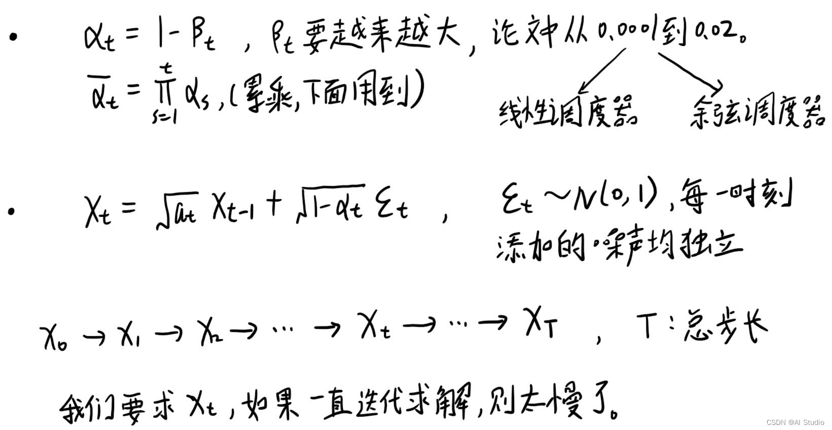
我们按照ddpm中用第二种的linear,将 t 设置为200,并将每个 t 下的各种参数提前计算好。
timesteps = 200

# define beta schedule
betas = linear_beta_schedule(timesteps=timesteps)

# define alphas
alphas = 1. - betas
alphas_cumprod = torch.cumprod(alphas, axis=0)
alphas_cumprod_prev = f.pad(alphas_cumprod[:-1], (1, 0), value=1.0)
sqrt_recip_alphas = torch.sqrt(1.0 / alphas)

# calculations for diffusion q(x_t | x_{t-1}) and others
sqrt_alphas_cumprod = torch.sqrt(alphas_cumprod)
sqrt_one_minus_alphas_cumprod = torch.sqrt(1. - alphas_cumprod)

# calculations for posterior q(x_{t-1} | x_t, x_0)
posterior_variance = betas * (1. - alphas_cumprod_prev) / (1. - alphas_cumprod)

def extract(a, t, x_shape):
    batch_size = t.shape[0]
    out = a.gather(-1, t.cpu())
    return out.reshape(batch_size, *((1,) * (len(x_shape) - 1))).to(t.device)
我们用一个实例来说明前向加噪过程。
from pil import image
import requests

url = 'http://images.cocodataset.org/val2017/000000039769.jpg'
image = image.open(requests.get(url, stream=true).raw)
image
from torchvision.transforms import compose, totensor, lambda, topilimage, centercrop, resize

image_size = 128
transform = compose([
    resize(image_size),
    centercrop(image_size),
    totensor(), # turn into numpy array of shape hwc, divide by 255
    lambda(lambda t: (t * 2) - 1),
])

x_start = transform(image).unsqueeze(0)
x_start.shape  # 输出的结果是 torch.size([1, 3, 128, 128])

import numpy as np

reverse_transform = compose([
     lambda(lambda t: (t + 1) / 2),
     lambda(lambda t: t.permute(1, 2, 0)), # chw to hwc
     lambda(lambda t: t * 255.),
     lambda(lambda t: t.numpy().astype(np.uint8)),
     topilimage(),
])
准备齐全,接下来就可以定义正向扩散过程了。
# forward diffusion (using the nice property)
def q_sample(x_start, t, noise=none):
    if noise is none:
        noise = torch.randn_like(x_start)

    sqrt_alphas_cumprod_t = extract(sqrt_alphas_cumprod, t, x_start.shape)
    sqrt_one_minus_alphas_cumprod_t = extract(
        sqrt_one_minus_alphas_cumprod, t, x_start.shape
    )

    return sqrt_alphas_cumprod_t * x_start + sqrt_one_minus_alphas_cumprod_t * noise

def get_noisy_image(x_start, t):
  # add noise
  x_noisy = q_sample(x_start, t=t)

  # turn back into pil image
  noisy_image = reverse_transform(x_noisy.squeeze())

  return noisy_image
可视化一下多个不同t的生成结果。
import matplotlib.pyplot as plt

# use seed for reproducability
torch.manual_seed(0)

# source: https://pytorch.org/vision/stable/auto_examples/plot_transforms.html#sphx-glr-auto-examples-plot-transforms-py
def plot(imgs, with_orig=false, row_title=none, **imshow_kwargs):
    if not isinstance(imgs[0], list):
        # make a 2d grid even if there's just 1 row
        imgs = [imgs]

    num_rows = len(imgs)
    num_cols = len(imgs[0]) + with_orig
    fig, axs = plt.subplots(figsize=(200,200), nrows=num_rows, ncols=num_cols, squeeze=false)
    for row_idx, row in enumerate(imgs):
        row = [image] + row if with_orig else row
        for col_idx, img in enumerate(row):
            ax = axs[row_idx, col_idx]
            ax.imshow(np.asarray(img), **imshow_kwargs)
            ax.set(xticklabels=[], yticklabels=[], xticks=[], yticks=[])

    if with_orig:
        axs[0, 0].set(title='original image')
        axs[0, 0].title.set_size(8)
    if row_title is not none:
        for row_idx in range(num_rows):
            axs[row_idx, 0].set(ylabel=row_title[row_idx])

    plt.tight_layout()

plot([get_noisy_image(x_start, torch.tensor([t])) for t in [0, 50, 100, 150, 199]])
3.8 定义损失函数
def p_losses(denoise_model, x_start, t, noise=none, loss_type="l1"):
    # 先采样噪声
    if noise is none:
        noise = torch.randn_like(x_start)

    # 用采样得到的噪声去加噪图片
    x_noisy = q_sample(x_start=x_start, t=t, noise=noise)
    predicted_noise = denoise_model(x_noisy, t)

    # 根据加噪了的图片去预测采样的噪声
    if loss_type == 'l1':
        loss = f.l1_loss(noise, predicted_noise)
    elif loss_type == 'l2':
        loss = f.mse_loss(noise, predicted_noise)
    elif loss_type == "huber":
        loss = f.smooth_l1_loss(noise, predicted_noise)
    else:
        raise notimplementederror()

    return loss
3.9 定义数据集 pytorch dataset 和 dataloader
我们使用mnist数据集构造了一个 dataloader,每个batch由128张 normalize 过的 image 组成。
from datasets import load_dataset

# load dataset from the hub
dataset = load_dataset("fashion_mnist")
image_size = 28
channels = 1
batch_size = 128


from torchvision import transforms
from torch.utils.data import dataloader

transform = compose([
            transforms.randomhorizontalflip(),
            transforms.totensor(),
            transforms.lambda(lambda t: (t * 2) - 1)
])

def transforms(examples):
   examples["pixel_values"] = [transform(image.convert("l")) for image in examples["image"]]
   del examples["image"]

   return examples

transformed_dataset = dataset.with_transform(transforms).remove_columns("label")
dataloader = dataloader(transformed_dataset["train"], batch_size=batch_size, shuffle=true)
batch = next(iter(dataloader))
print(batch.keys())    # dict_keys(['pixel_values'])
3.10 采样
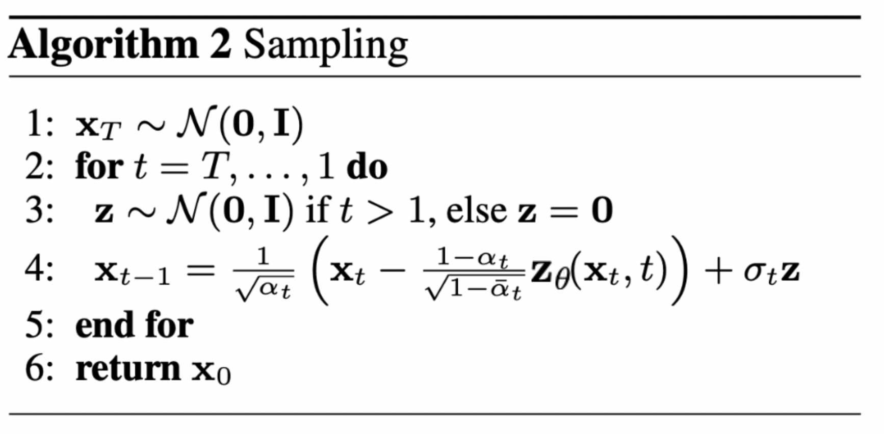
采样过程发生在反向去噪时。对于一张纯噪声,扩散模型一步步地去除噪声最终得到真实图片,采样事实上就是定义的去除噪声这一行为。 观察采样算法中第四行, t−1 步的图片是由 t 步的图片减去一个噪声得到的,只不过这个噪声是由网络拟合出来,并且 rescale 过的而已。 这里要注意第四行式子的最后一项,采样时每一步也都会加上一个从正态分布采样的纯噪声。理想情况下,最终我们会得到一张看起来像是从真实数据分布中采样得到的图片。
@torch.no_grad()
def p_sample(model, x, t, t_index):
    betas_t = extract(betas, t, x.shape)
    sqrt_one_minus_alphas_cumprod_t = extract(
        sqrt_one_minus_alphas_cumprod, t, x.shape
    )
    sqrt_recip_alphas_t = extract(sqrt_recip_alphas, t, x.shape)

    # equation 11 in the paper
    # use our model (noise predictor) to predict the mean
    model_mean = sqrt_recip_alphas_t * (
        x - betas_t * model(x, t) / sqrt_one_minus_alphas_cumprod_t
    )

    if t_index == 0:
        return model_mean
    else:
        posterior_variance_t = extract(posterior_variance, t, x.shape)
        noise = torch.randn_like(x)
        # algorithm 2 line 4:
        return model_mean + torch.sqrt(posterior_variance_t) * noise

# algorithm 2 (including returning all images)
@torch.no_grad()
def p_sample_loop(model, shape):
    device = next(model.parameters()).device

    b = shape[0]
    # start from pure noise (for each example in the batch)
    img = torch.randn(shape, device=device)
    imgs = []

    for i in tqdm(reversed(range(0, timesteps)), desc='sampling loop time step', total=timesteps):
        img = p_sample(model, img, torch.full((b,), i, device=device, dtype=torch.long), i)
        imgs.append(img.cpu().numpy())
    return imgs

@torch.no_grad()
def sample(model, image_size, batch_size=16, channels=3):
    return p_sample_loop(model, shape=(batch_size, channels, image_size, image_size))
3.11 训练
先定义一些辅助生成图片的函数。
from pathlib import path

def num_to_groups(num, divisor):
    groups = num // divisor
    remainder = num % divisor
    arr = [divisor] * groups
    if remainder > 0:
        arr.append(remainder)
    return arr

results_folder = path("./results")
results_folder.mkdir(exist_ok = true)
save_and_sample_every = 1000
接下来实例化模型。
from torch.optim import adam

device = "cuda" if torch.cuda.is_available() else "cpu"

model = unet(
    dim=image_size,
    channels=channels,
    dim_mults=(1, 2, 4,)
)
model.to(device)

optimizer = adam(model.parameters(), lr=1e-3)
开始训练!
from torchvision.utils import save_image

epochs = 6

for epoch in range(epochs):
    for step, batch in enumerate(dataloader):
      optimizer.zero_grad()

      batch_size = batch["pixel_values"].shape[0]
      batch = batch["pixel_values"].to(device)

      # algorithm 1 line 3: sample t uniformally for every example in the batch
      t = torch.randint(0, timesteps, (batch_size,), device=device).long()

      loss = p_losses(model, batch, t, loss_type="huber")

      if step % 100 == 0:
        print("loss:", loss.item())

      loss.backward()
      optimizer.step()

      # save generated images
      if step != 0 and step % save_and_sample_every == 0:
        milestone = step // save_and_sample_every
        batches = num_to_groups(4, batch_size)
        all_images_list = list(map(lambda n: sample(model, batch_size=n, channels=channels), batches))
        all_images = torch.cat(all_images_list, dim=0)
        all_images = (all_images + 1) * 0.5
        save_image(all_images, str(results_folder / f'sample-{milestone}.png'), nrow = 6)
inference:
# sample 64 images
samples = sample(model, image_size=image_size, batch_size=64, channels=channels)

# show a random one
random_index = 5
plt.imshow(samples[-1][random_index].reshape(image_size, image_size, channels), cmap="gray")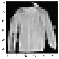
import matplotlib.animation as animation

random_index = 53

fig = plt.figure()
ims = []
for i in range(timesteps):
    im = plt.imshow(samples[i][random_index].reshape(image_size, image_size, channels), cmap="gray", animated=true)
    ims.append([im])

animate = animation.artistanimation(fig, ims, interval=50, blit=true, repeat_delay=1000)
animate.save('diffusion.gif')
plt.show()
4. 参考文献


发表评论