Python图像处理之二值化处理_Python

1、什么是二值化处理

我们都知道，图像是由矩阵构成，矩阵中每个点的rgb值都不一样，呈现出来的色彩不一样，最终整体呈现给我们的就是一张彩色的图像。所谓”二值化处理“就是将矩阵中每个点的rgb值（0，0，0）[黑色]或者（255，255，255）[白色]

2、为什么要进行二值化处理

早期人们使用计算机处理图像是，实在图像灰度化处理的基础上在进行操作的，但是当时的硬件水平不足，所以处理速度很慢，于是人们引入了图像二值化处理。二值化处理使得原本颜色的取值范围从256种变为2种，确实是提高了计算速度，但是丢失的信息也多了，因此具体采用什么方式处理，要根据具体情况来选择。

3、如何进行二值化处理

（1）简单阈值

简单阈值是选取一个全局阈值，然后把整幅图像分成非黑即白的二值图像，灰度值大于阈值就赋为255反之为0。

ret,mask = cv2.threshold(img2gray,175,255,cv2.thresh_binar)

返回值一：阈值，（otsu‘s二值化会用到）
返回值二：处理以后的图像
参数一: 初始图像
参数二：我们自己设定的阈值
参数三：当图像像素置超过我们的设定的阈值时赋为255
参数四 : 我们设定的二值化类型

阈值	小于阈值	大于阈值
thresh_binary	置0	置填充色
thresh_binary_inv	置填充色	0
thresh_trunc	保持原色	置灰色
thresh_tozero	置0	保持原色
thresh_tozero_inv	保持原色	置0

注：cv2.threshold最后一个参数可以写为0，1，2，3，4按顺序对应表格中的五种
代码如下

import cv2
import matplotlib.pyplot as plt
img = cv2.imread('dog.jpeg', 0)  # 直接读为灰度图像
ret, thresh1 = cv2.threshold(img, 127, 255, 0)
ret, thresh2 = cv2.threshold(img, 127, 255, 1)
ret, thresh3 = cv2.threshold(img, 127, 255, 2)
ret, thresh4 = cv2.threshold(img, 127, 255, 3)
ret, thresh5 = cv2.threshold(img, 127, 255, 4)
titles = ['img', 'binary', 'binary_inv', 'trunc', 'tozero', 'tozero_inv']
images = [img, thresh1, thresh2, thresh3, thresh4, thresh5]
for i in range(6):
    plt.subplot(2, 3, i + 1), plt.imshow(images[i],'gray')
    plt.title(titles[i])
    plt.xticks([]), plt.yticks([])
plt.show()

在这里插入图片描述

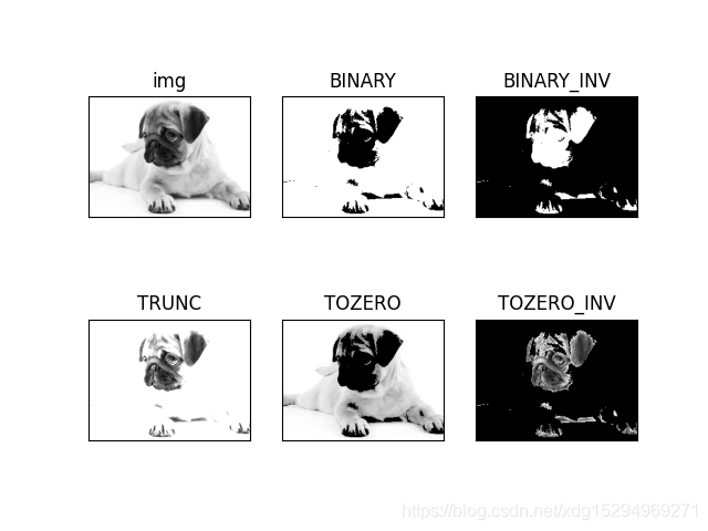
注：将阈值大于127的像素值置为255

（2）自适应阈值

简单阈值的方式过于粗鲁，自适应阈值更趋向于局部性的阈值，也就是说，将像素点的像素值与该点所在的区域的像素值的平均值（最大值，中位数等）决定该店属于0还是1

th2 = cv.adaptivethreshold(img,255,cv.adaptive_thresh_mean_c,0,11,2)

返回值: 处理后返回的图像
参数一：原始图像
参数二：像素值上限
参数三：自适应方法
— cv2.adaptive_thresh_mean_c ：领域内均值
—cv2.adaptive_thresh_gaussian_c ：领域内像素点加权和
参数四：赋值方式（参考简单阈值中介绍的表格）
参数五：设定方阵的大小（因为是将一个点与其周围的方阵数据对比）
参数六：常数，每个区域计算出的阈值的基础上在减去这个常数作为这个区域的最终阈值，可以为负数

import cv2 as cv
import numpy as np
from matplotlib import pyplot as plt
img = cv.imread('dog.jpeg',0)
img = cv.medianblur(img,5)
ret,th1 = cv.threshold(img,127,255,cv.thresh_binary)
th2 = cv.adaptivethreshold(img,255,cv.adaptive_thresh_mean_c,0,11,2)
th3 = cv.adaptivethreshold(img,255,cv.adaptive_thresh_gaussian_c,0,11,2)
titles = ['original image', 'global thresholding (v = 127)',
            'adaptive mean thresholding', 'adaptive gaussian thresholding']
images = [img, th1, th2, th3]
for i in range(4):
    plt.subplot(2,2,i+1),plt.imshow(images[i],'gray')
    plt.title(titles[i])
    plt.xticks([]),plt.yticks([])
plt.show()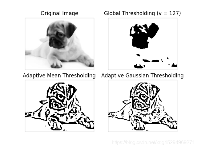

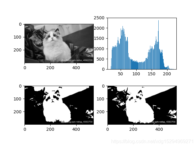
在这里插入图片描述

（3）otsu’s二值化

对于简单阈值，cv2.threshold()的第二个参数是我们自己设定的阈值范围，一张图片的最好的阈值分界线不是凭感觉看出来的，而是有合理的方式能找到的，threshold的第一个返回值就是处理图片的阈值分界线。因此，只要在threshold函数的最后一个参数在原有的基础上加上’cv2.thresh_otsu‘那么第一个返回值就是最佳阈值。直接看代码更好理解。
注：otsu非常适合灰度直方图具有双峰值的情况

import cv2
import matplotlib.pyplot as plt
img = cv2.imread('cat.jpg', 0)  # 直接读为灰度图像
# 简单滤波
ret1, th1 = cv2.threshold(img, 127, 255, cv2.thresh_binary)
print(ret1)
# otsu 滤波
ret2, th2 = cv2.threshold(img, 0, 255, cv2.thresh_binary + cv2.thresh_otsu)
print(ret2)
plt.figure()
plt.subplot(221), plt.imshow(img,'gray')
plt.subplot(222), plt.hist(img.ravel(), 256)  # .ravel方法将矩阵转化为一维
plt.subplot(223), plt.imshow(th1,'gray')
plt.subplot(224), plt.imshow(th2,'gray')
plt.show()

在这里插入图片描述

4、参考文献：

https://numpy.org/doc/stable/reference/generated/numpy.hstack.html
https://zhuanlan.zhihu.com/p/360824614
https://blog.csdn.net/jjddss/article/details/72841
https://blog.csdn.net/li_l_il/article/details/86767790
https://blog.csdn.net/jningwei/article/details/77747959
https://blog.csdn.net/weixin_35732969/article/details/83779660

声明：部分图像源自网络，本文仅供学习交流使用，如果不妥，请联系删除。

到此这篇关于python图像处理之二值化处理的文章就介绍到这了,更多相关python二值化处理内容请搜索代码网以前的文章或继续浏览下面的相关文章希望大家以后多多支持代码网！