一文详解如何在Python中进行数学建模_Python

数学建模是数据科学中使用的强大工具，通过数学方程和算法来表示真实世界的系统和现象。python拥有丰富的库生态系统，为开发和实现数学模型提供了一个很好的平台。本文将指导您完成python中的数学建模过程，重点关注数据科学中的应用。

数学建模导论

数学建模是将现实世界中的问题用数学术语表示的过程。它涉及定义变量、方程和约束来模拟或预测复杂系统的行为。这些模型可用于模拟、分析和预测复杂系统的行为。

在数据科学中，数学模型对于回归分析、分类、聚类、优化等任务至关重要。python及其丰富的库生态系统为数学建模提供了强大的平台。

在python中进行数学建模的步骤：

问题表述：明确定义模型想要解决的问题。确定所涉及的相关变量、参数和关系。

制定模型：一旦问题被定义，下一步就是制定数学模型。这涉及到将现实世界的问题转化为数学方程。您选择的模型类型将取决于问题的性质。常见的模型类型包括：

线性模型：用于变量之间的关系是线性的问题。

非线性模型：用于具有非线性关系的问题。

微分方程：用于建模随时间变化的动态系统。

随机模型：用于涉及随机性或不确定性的系统。

实现：在编程环境中实现数学模型。这一步包括编写代码来表示方程并用数值求解它们。

验证和分析：通过将模型的预测与真实世界的数据或实验结果进行比较来验证模型。分析模型在不同条件和参数下的行为。

为什么使用python进行数学建模

python是数学建模的热门选择，因为它的简单性，可读性和广泛的库支持。数学建模中使用的一些关键库包括：

numpy：提供对大型多维数组和矩阵的支持，沿着对这些数组进行操作的数学函数集合。

scipy：基于numpy构建，为科学和技术计算提供额外的功能，包括优化、积分、插值、特征值问题等。

sympy：一个符号数学库，允许代数操作，微积分和方程求解。

matplotlib：一个绘图库，用于创建静态、动画和交互式可视化。

pandas：一个数据操作和分析库，提供无缝处理结构化数据所需的数据结构和函数。

python中的数学建模技术

python提供了几个库和工具，用于跨各个领域的数学建模。以下是一些流行的技术和相应的库：

微分方程：使用scipy、sympy和differentialequations.jl（通过pycall）等库求解常微分方程和偏微分方程。

优化：使用scipy，cvxpy和pulp等库进行优化和约束满足。

simulation：使用simpy（用于离散事件仿真）和pydstool（用于动态系统）等库模拟动态系统。

统计建模：使用statsmodels、scikit-learn和pymc 3等库将统计模型拟合到数据，以进行贝叶斯建模。

示例1：求解微分方程

让我们通过求解微分方程的简单示例来说明python中数学建模的过程：

import numpy as np
from scipy.integrate import solve_ivp
import matplotlib.pyplot as plt
# define the differential equation
def damped_oscillator(t, y):
    return [y[1], -0.1 * y[1] - np.sin(y[0])]
initial_conditions = [0, 1]
t_span = (0, 20)
# solve the differential equation
solution = solve_ivp(damped_oscillator, t_span, initial_conditions)
# plot the solution
plt.plot(solution.t, solution.y[0])
plt.xlabel('time')
plt.ylabel('position')
plt.title('damped oscillator')
plt.show()

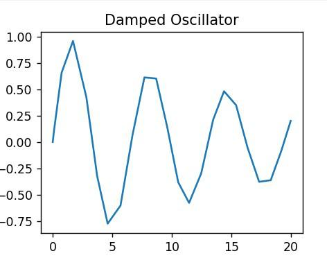
在这个例子中，我们定义了一个阻尼振荡器，微分方程指定了初始条件和时间跨度，使用scipy中的solve_ivp求解方程，并使用matplotlib绘制解。

示例2：使用scipy进行非线性优化

非线性优化涉及优化非线性目标函数。在这里，我们使用scipy来解决一个非线性优化问题。

import numpy as np
from scipy.optimize import minimize

# define the objective function
def objective(x):
    return (x[0] - 2)**2 + (x[1] - 3)**2

# define the constraints
constraints = [{'type': 'ineq', 'fun': lambda x: 5 - (x[0] + x[1])},
               {'type': 'ineq', 'fun': lambda x: x[0]},
               {'type': 'ineq', 'fun': lambda x: x[1]}]

# define the initial guess
x0 = np.array([0, 0])

# solve the problem
result = minimize(objective, x0, constraints=constraints)

# print the results
print(f"status: {result.success}")
print(f"x = {result.x}")
print(f"objective value = {result.fun}")

输出

status: true
x = [1.99999999 2.99999999]
objective value = 1.4388348792344465e-16

示例3：使用simpy进行离散事件模拟

离散事件仿真将系统的操作建模为时间上的事件序列。在这里，我们使用simpy来模拟一个简单的队列系统。

安装：

pip install simpy

代码：

import simpy
import random

def customer(env, name, counter, service_time):
    print(f'{name} arrives at the counter at {env.now:.2f}')
    with counter.request() as request:
        yield request
        print(f'{name} starts being served at {env.now:.2f}')
        yield env.timeout(service_time)
        print(f'{name} leaves the counter at {env.now:.2f}')

def setup(env, num_counters, service_time, arrival_interval):
    counter = simpy.resource(env, num_counters)
    for i in range(5):
        env.process(customer(env, f'customer {i}', counter, service_time))
    while true:
        yield env.timeout(random.expovariate(1.0 / arrival_interval))
        i += 1
        env.process(customer(env, f'customer {i}', counter, service_time))

# initialize the environment
env = simpy.environment()
env.process(setup(env, num_counters=1, service_time=5, arrival_interval=10))

# run the simulation
env.run(until=50)

输出

customer 0 arrives at the counter at 0.00
customer 1 arrives at the counter at 0.00
customer 2 arrives at the counter at 0.00
customer 3 arrives at the counter at 0.00
customer 4 arrives at the counter at 0.00
customer 0 starts being served at 0.00
customer 0 leaves the counter at 5.00
customer 1 starts being served at 5.00
customer 1 leaves the counter at 10.00
customer 2 starts being served at 10.00
customer 5 arrives at the counter at 12.90
customer 2 leaves the counter at 15.00
customer 3 starts being served at 15.00
customer 6 arrives at the counter at 17.87
customer 7 arrives at the counter at 18.92
customer 3 leaves the counter at 20.00
customer 4 starts being served at 20.00
customer 8 arrives at the counter at 24.37
customer 4 leaves the counter at 25.00
customer 5 starts being served at 25.00
customer 5 leaves the counter at 30.00
customer 6 starts being served at 30.00
customer 9 arrives at the counter at 31.08
customer 10 arrives at the counter at 32.16
customer 6 leaves the counter at 35.00
customer 7 starts being served at 35.00
customer 11 arrives at the counter at 36.80
customer 7 leaves the counter at 40.00
customer 8 starts being served at 40.00
customer 8 leaves the counter at 45.00
customer 9 starts being served at 45.00
customer 12 arrives at the counter at 45.34

示例4：使用statsmodels的线性回归

线性回归是一种统计方法，用于对因变量与一个或多个自变量之间的关系进行建模。在这里，我们使用statsmodels来执行线性回归。

import statsmodels.api as sm
import numpy as np

# generate random data
np.random.seed(0)
x = np.random.rand(100, 1)
y = 3 * x.squeeze() + 2 + np.random.randn(100)

# add a constant to the independent variables
x = sm.add_constant(x)

# fit the model
model = sm.ols(y, x).fit()

# print the results
print(model.summary())

输出

ols regression results
==============================================================================
dep. variable: y r-squared: 0.419
model: ols adj. r-squared: 0.413
method: least squares f-statistic: 70.80
date: tue, 18 jun 2024 prob (f-statistic): 3.29e-13
time: 08:16:41 log-likelihood: -141.51
no. observations: 100 aic: 287.0
df residuals: 98 bic: 292.2
df model: 1
covariance type: nonrobust
==============================================================================
coef std err t p>|t| [0.025 0.975]
------------------------------------------------------------------------------
const 2.2222 0.193 11.496 0.000 1.839 2.606
x1 2.9369 0.349 8.414 0.000 2.244 3.630
==============================================================================
omnibus: 11.746 durbin-watson: 2.083
prob(omnibus): 0.003 jarque-bera (jb): 4.097
skew: 0.138 prob(jb): 0.129
kurtosis: 2.047 cond. no. 4.30
==============================================================================