利用【MATLAB】和【Python】进行【图与网络模型】的高级应用与分析】

一、图与网络的基本概念

1. 无向图与有向图

• 无向图：由顶点集合和边集合组成，边是无方向的。表示为 g=(v,e)，其中 v 是顶点集合， e 是边集合。
• 有向图：边是有方向的，从一个顶点指向另一个顶点。表示为 g=(v,e)，其中每条边用有序对表示。

2. 简单图、完全图、赋权图

• 简单图：无重复边和自环的图。
• 完全图：每对顶点之间都有边的图， kn​ 表示n个顶点的完全图。
• 赋权图：边带有权值的图，用于表示边的某种属性，如距离、费用等。

3. 顶点的度

• 度：与顶点相连的边的数目。在无向图中，顶点的度即为相连边的数目。在有向图中，入度为指向该顶点的边数，出度为从该顶点出发的边数。

4. 子图与连通性

• 子图：由原图的一部分顶点和边组成的图。
• 连通性：图中任意两顶点之间存在路径。无向图称为连通图，有向图称为强连通图。

5. 图的矩阵表示

• 邻接矩阵：表示顶点之间是否有边的矩阵。若顶点 i 和顶点 j 之间有边，则矩阵a[i][j] 为1，否则为0。
• 关联矩阵：表示顶点和边关系的矩阵。若边ek​ 连接顶点 vi​ 和 vj​，则矩阵 a[i][k] 和]a[j][k] 分别为1。

matlab代码实例

% matlab代码
% 创建无向图和有向图的邻接矩阵表示

% 无向图的邻接矩阵
a_undirected = [0 1 1 0; 
                1 0 1 1; 
                1 1 0 1; 
                0 1 1 0];

% 有向图的邻接矩阵
a_directed = [0 1 0 0; 
              0 0 1 0; 
              0 0 0 1; 
              1 0 0 0];

% 显示邻接矩阵
disp('无向图的邻接矩阵:');
disp(a_undirected);

disp('有向图的邻接矩阵:');
disp(a_directed);

% 创建图对象并可视化
g_undirected = graph(a_undirected);
g_directed = digraph(a_directed);

% 绘制图
figure;
subplot(1,2,1);
plot(g_undirected);
title('无向图');

subplot(1,2,2);
plot(g_directed);
title('有向图');

无向图的邻接矩阵:
     0     1     1     0
     1     0     1     1
     1     1     0     1
     0     1     1     0

有向图的邻接矩阵:
     0     1     0     0
     0     0     1     0
     0     0     0     1
     1     0     0     0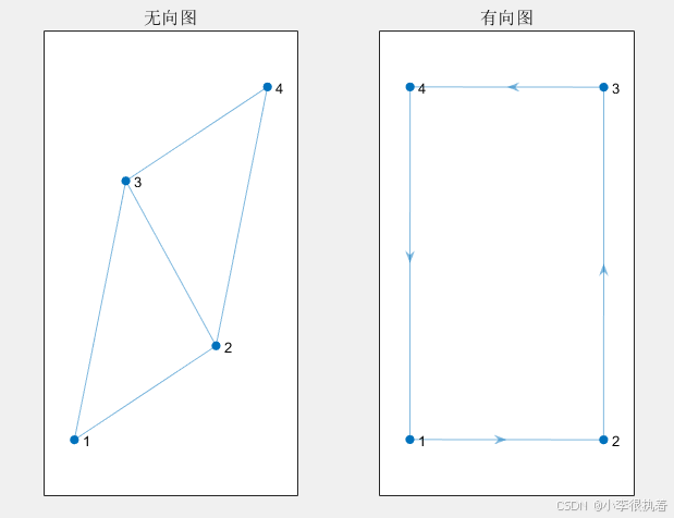

邻接矩阵表示

无向图的邻接矩阵：a_undirected 是一个4x4矩阵，其中 a_undirected(i, j) 表示顶点 i 和顶点 j 之间是否有边。对于无向图，矩阵是对称的。
有向图的邻接矩阵：a_directed 是一个4x4矩阵，其中 a_directed(i, j) 表示顶点 i 到顶点 j 之间是否有边。对于有向图，矩阵不是对称的。
显示邻接矩阵

使用 disp 函数显示无向图和有向图的邻接矩阵，以便于检查矩阵的正确性。
创建图对象并可视化

graph(a_undirected) 创建无向图对象。
digraph(a_directed) 创建有向图对象。
使用 plot 函数可视化图对象。subplot 函数将图分成两部分，分别显示无向图和有向图。

python代码实例 

import networkx as nx
import matplotlib.pyplot as plt
import numpy as np
from matplotlib.font_manager import fontproperties

# 设置中文字体
font = fontproperties(fname=r"c:\windows\fonts\simsun.ttc", size=15)

# 无向图的邻接矩阵
a_undirected = np.array([
    [0, 1, 1, 0],
    [1, 0, 1, 1],
    [1, 1, 0, 1],
    [0, 1, 1, 0]
])

# 有向图的邻接矩阵
a_directed = np.array([
    [0, 1, 0, 0],
    [0, 0, 1, 0],
    [0, 0, 0, 1],
    [1, 0, 0, 0]
])

# 使用邻接矩阵创建无向图和有向图
g_undirected = nx.from_numpy_array(a_undirected)
g_directed = nx.from_numpy_array(a_directed, create_using=nx.digraph)

# 绘制无向图
plt.figure(figsize=(10, 5))
plt.subplot(1, 2, 1)
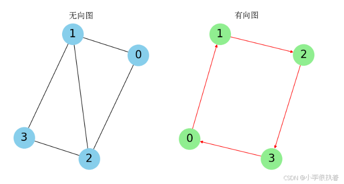
nx.draw(g_undirected, with_labels=true, node_color='skyblue', edge_color='black', node_size=1500, font_size=20)
plt.title('无向图', fontproperties=font)

# 绘制有向图
plt.subplot(1, 2, 2)
nx.draw(g_directed, with_labels=true, node_color='lightgreen', edge_color='red', node_size=1500, font_size=20, arrows=true)
plt.title('有向图', fontproperties=font)

plt.show()

注意的细节知识点

邻接矩阵表示

确保邻接矩阵的对称性（对于无向图）。
邻接矩阵的大小应为 n x n，其中 n 是顶点数量。
显示矩阵

使用 disp 或 print 函数显示矩阵，便于检查矩阵的正确性。
创建图对象

使用 graph 和 digraph 函数分别创建无向图和有向图对象。
确保输入的邻接矩阵符合图的类型（无向或有向）。
可视化图

使用 plot 函数可视化图对象，便于直观理解图的结构。
在python中，可以使用 networkx 库中的 draw 函数进行可视化，matplotlib 库中的 subplot 函数分割图形窗口。
matlab和python的差异

matlab中的 graph 和 digraph 函数对应于python中的 nx.graph 和 nx.digraph。
matlab中的 disp 函数对应于python中的 print 函数。
matlab中的 plot 函数对应于python中的 nx.draw 函数。

二、最短路径问题

1. 最短路径问题的定义

• 最短路径问题是寻找从一个顶点到另一个顶点的路径，使得路径上的边权值和最小。

2. dijkstra算法

• 适用于非负权图的单源最短路径问题。
• 算法步骤：

matlab代码实例

% matlab代码
% dijkstra算法实现
function [dist, path] = dijkstra(a, start_node)
    n = size(a, 1); % 顶点数量
    dist = inf(1, n); % 初始化距离
    dist(start_node) = 0;
    visited = false(1, n); % 访问标记
    path = -ones(1, n); % 路径
    
    for i = 1:n
        % 选择未处理顶点中距离最小的顶点
        [~, u] = min(dist + visited * inf);
        visited(u) = true;
        
        % 更新邻接顶点的距离
        for v = 1:n
            if a(u, v) > 0 && ~visited(v)
                alt = dist(u) + a(u, v);
                if alt < dist(v)
                    dist(v) = alt;
                    path(v) = u;
                end
            end
        end
    end
end

% 示例图的邻接矩阵
a = [0 10 20 0 0;
     10 0 5 1 0;
     20 5 0 2 3;
     0 1 2 0 4;
     0 0 3 4 0];

% 计算从起点1到其他顶点的最短路径
[start_node] = 1;
[dist, path] = dijkstra(a, start_node);

% 显示结果
disp('顶点的最短距离:');
disp(dist);
disp('最短路径:');
disp(path);

% 可视化结果
g = digraph(a);
figure;
h = plot(g, 'edgelabel', g.edges.weight);
highlight(h, path, 'edgecolor', 'r', 'linewidth', 2);
title('dijkstra最短路径');

顶点的最短距离:
     0    10    20   inf   inf

最短路径:
    -1     1     1    -1    -1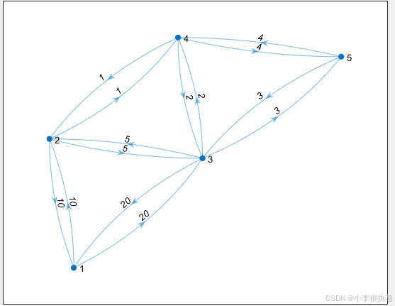

初始化

n = size(a, 1)：获取图中顶点的数量。
dist = inf(1, n)：初始化每个顶点的距离为无穷大。
dist(start_node) = 0：起点到自身的距离为0。
visited = false(1, n)：初始化访问标记。
path = -ones(1, n)：初始化路径数组。
主循环

for i = 1:n：对每个顶点进行迭代。
[~, u] = min(dist + visited * inf)：选择未处理顶点中距离最小的顶点。
visited(u) = true：将该顶点标记为已处理。
更新邻接顶点的距离

for v = 1:n：对每个邻接顶点进行迭代。
if a(u, v) > 0 && ~visited(v)：如果顶点 v 与顶点 u 之间有边且未被访问。
alt = dist(u) + a(u, v)：计算通过顶点 u 到顶点 v 的距离。
if alt < dist(v)：如果通过 u 到 v 的距离小于当前已知的 v 的距离。
dist(v) = alt：更新 v 的距离。
path(v) = u：更新 v 的路径。

python代码实例

import heapq

def dijkstra(a, start_node):
    n = len(a)
    dist = [float('inf')] * n
    dist[start_node] = 0
    visited = [false] * n
    path = [-1] * n
    queue = [(0, start_node)]
    
    while queue:
        d, u = heapq.heappop(queue)
        if visited[u]:
            continue
        visited[u] = true
        
        for v, weight in enumerate(a[u]):
            if weight > 0 and not visited[v]:
                alt = dist[u] + weight
                if alt < dist[v]:
                    dist[v] = alt
                    path[v] = u
                    heapq.heappush(queue, (alt, v))
    
    return dist, path

# 示例图的邻接矩阵
a = [
    [0, 10, 20, 0, 0],
    [10, 0, 5, 1, 0],
    [20, 5, 0, 2, 3],
    [0, 1, 2, 0, 4],
    [0, 0, 3, 4, 0]
]

# 计算从起点0到其他顶点的最短路径
start_node = 0
dist, path = dijkstra(a, start_node)

# 显示结果
print('顶点的最短距离:', dist)
print('最短路径:', path)

顶点的最短距离: [0, 10, 13, 11, 15]
最短路径: [-1, 0, 3, 1, 3]

三、最小生成树问题

1. 最小生成树的定义

• 最小生成树（mst）是包含图中所有顶点且边权值和最小的生成树。

2. kruskal算法

• 适用于任意图。
• 算法步骤：
  1. 将图中的边按权值从小到大排序。
  2. 依次选择权值最小的边，若该边的加入不形成圈，则将其加入生成树。
  3. 重复步骤2，直到生成树包含所有顶点。

matlab代码实例

% matlab代码
% kruskal算法实现
function [mst_edges, mst_weight] = kruskal(a)
    n = size(a, 1);
    edges = [];
    for i = 1:n
        for j = i+1:n
            if a(i, j) > 0
                edges = [edges; i, j, a(i, j)];
            end
        end
    end
    edges = sortrows(edges, 3);
    
    parent = 1:n;
    mst_edges = [];
    mst_weight = 0;
    
    function p = find(parent, x)
        if parent(x) == x
            p = x;
        else
            p = find(parent, parent(x));
            parent(x) = p;
        end
    end

    for k = 1:size(edges, 1)
        u = edges(k, 1);
        v = edges(k, 2);
        w = edges(k, 3);
        pu = find(parent, u);
        pv = find(parent, v);
        if pu ~= pv
            mst_edges = [mst_edges; u, v];
            mst_weight = mst_weight + w;
            parent(pu) = pv;
        end
    end
end

% 示例图的邻接矩阵
a = [0 10 6 5;
     10 0 0 15;
     6 0 0 4;
     5 15 4 0];

% 计算最小生成树
[mst_edges, mst_weight] = kruskal(a);

% 显示结果
disp('最小生成树的边:');
disp(mst_edges);
disp('最小生成树的权重:');
disp(mst_weight);

% 可视化结果
g = graph(a);
figure;
h = plot(g, 'edgelabel', g.edges.weight);
highlight(h, mst_edges(:,1), mst_edges(:,2), 'edgecolor', 'r', 'linewidth', 2);
title('kruskal最小生成树');

最小生成树的边:
     3     4
     1     4
     1     2

最小生成树的权重:
    19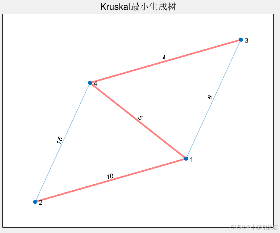

初始化

n = size(a, 1)：获取图中顶点的数量。
edges = []：初始化边的列表。
使用嵌套循环遍历邻接矩阵，收集所有边的信息。
边的排序

edges = sortrows(edges, 3)：按边的权值从小到大排序。
并查集的初始化

parent = 1:n：初始化每个顶点的父节点为自身。
mst_edges = []：初始化最小生成树的边列表。
mst_weight = 0：初始化最小生成树的权重和。
并查集查找函数

function p = find(parent, x)：递归查找顶点的根节点，并进行路径压缩。

python代码实例

class unionfind:
    def __init__(self, n):
        self.parent = list(range(n))
    
    def find(self, u):
        if self.parent[u] != u:
            self.parent[u] = self.find(self.parent[u])
        return self.parent[u]
    
    def union(self, u, v):
        root_u = self.find(u)
        root_v = self.find(v)
        if root_u != root_v:
            self.parent[root_u] = root_v

def kruskal(a):
    n = len(a)
    edges = [(a[i][j], i, j) for i in range(n) for j in range(i + 1, n) if a[i][j] > 0]
    edges.sort()
    
    uf = unionfind(n)
    mst_edges = []
    mst_weight = 0
    
    for weight, u, v in edges:
        if uf.find(u) != uf.find(v):
            uf.union(u, v)
            mst_edges.append((u, v))
            mst_weight += weight
    
    return mst_edges, mst_weight

# 示例图的邻接矩阵
a = [
    [0, 10, 6, 5],
    [10, 0, 0, 15],
    [6, 0, 0, 4],
    [5, 15, 4, 0]
]

# 计算最小生成树
mst_edges, mst_weight = kruskal(a)

# 显示结果
print('最小生成树的边:', mst_edges)
print('最小生成树的权重:', mst_weight)

注意的细节知识点

四、钢管订购和运输问题

1. 问题描述

• 需要从多个钢厂订购钢管，并将其运输到施工地点，铺设天然气主管道。
• 图中表示钢厂、枢纽点和施工地点，边的权值表示运输距离。

2. 问题分析

• 分解为两个子问题：从钢厂到枢纽点的运输和从枢纽点到施工地点的铺设。

• 需要综合考虑订购费用、运输费用和铺设费用。

3. 模型的建立与求解

• 运费矩阵的计算模型：计算从供应点到需求点的最小购运费。
• 总费用的数学规划模型：包括订购费用、运输费用和铺设管道的运费。
• 模型求解：利用floyd算法计算最短路径，运用数学规划模型优化总费用。

matlab代码实例

% matlab代码
% 构造铁路距离赋权图
function dist = floyd_warshall(a)
    n = size(a, 1);
    dist = a;
    dist(dist == 0) = inf;
    dist(1:n+1:end) = 0;
    for k = 1:n
        for i = 1:n
            for j = 1:n
                if dist(i, k) + dist(k, j) < dist(i, j)
                    dist(i, j) = dist(i, k) + dist(k, j);
                end
            end
        end
    end
end

% 示例图的邻接矩阵
a = [0 10 inf inf inf;
     10 0 5 inf inf;
     inf 5 0 3 inf;
     inf inf 3 0 1;
     inf inf inf 1 0];

% 计算最短路径
dist = floyd_warshall(a);

% 计算总费用的数学规划模型
function total_cost = steel_pipeline_optimization(supplies, demands, cost_matrix)
    n_suppliers = length(supplies);
    n_demands = length(demands);
    total_cost = 0;
    for i = 1:n_suppliers
        for j = 1:n_demands
            total_cost = total_cost + supplies(i) * cost_matrix(i, j);
        end
    end
end

% 示例数据
supplies = [100, 200, 150];
demands = [50, 100, 200, 100];
cost_matrix = [2, 4, 5, 6;
               3, 2, 7, 4;
               6, 5, 2, 3];

% 计算总费用
total_cost = steel_pipeline_optimization(supplies, demands, cost_matrix);

% 显示结果
disp('总费用:');
disp(total_cost);

% 可视化结果
figure;
imagesc(dist);
colorbar;
title('floyd-warshall最短路径距离矩阵');
xlabel('目标节点');
ylabel('起始节点');

python代码实例 

import numpy as np

def floyd_warshall(a):
    n = len(a)
    dist = np.array(a, dtype=float)
    dist[dist == 0] = np.inf
    np.fill_diagonal(dist, 0)
    for k in range(n):
        for i in range(n):
            for j in range(n):
                if dist[i, k] + dist[k, j] < dist[i, j]:
                    dist[i, j] = dist[i, k] + dist[k, j]
    return dist

# 示例图的邻接矩阵
a = [
    [0, 10, float('inf'), float('inf'), float('inf')],
    [10, 0, 5, float('inf'), float('inf')],
    [float('inf'), 5, 0, 3, float('inf')],
    [float('inf'), float('inf'), 3, 0, 1],
    [float('inf'), float('inf'), float('inf'), 1, 0]
]

# 计算最短路径
dist = floyd_warshall(a)

def steel_pipeline_optimization(supplies, demands, cost_matrix):
    total_cost = 0
    for i in range(len(supplies)):
        for j in range(len(demands)):
            total_cost += supplies[i] * cost_matrix[i][j]
    return total_cost

# 示例数据
supplies = [100, 200, 150]
demands = [50, 100, 200, 100]
cost_matrix = [
    [2, 4, 5, 6],
    [3, 2, 7, 4],
    [6, 5, 2, 3]
]

# 计算总费用
total_cost = steel_pipeline_optimization(supplies, demands, cost_matrix)

# 显示结果
print('总费用:', total_cost)

总费用: 7300

五、matlab工具箱的应用

1. matlab在图与网络中的应用

• matlab提供了强大的工具箱，用于处理图与网络问题。通过编写脚本和函数，可以实现图的生成、算法的实现及结果的可视化。

matlab代码实例

% 创建图对象并可视化
g = graph([1 2 2 3 3 4 4 5 5], [2 3 4 4 5 5 1 1 2], [10 20 30 40 50 60 70 80 90]);

% 可视化图
figure;
plot(g, 'edgelabel', g.edges.weight);
title('图的可视化');

% 计算最短路径
[start_node, end_node] = deal(1, 5);
[dist, path] = shortestpath(g, start_node, end_node);

% 显示最短路径
disp('最短路径:');
disp(path);

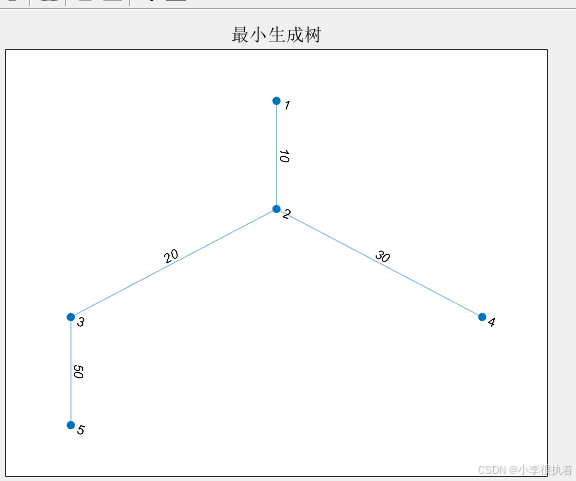
% 计算最小生成树
t = minspantree(g);
figure;
plot(t, 'edgelabel', t.edges.weight);
title('最小生成树');

最短路径:
    80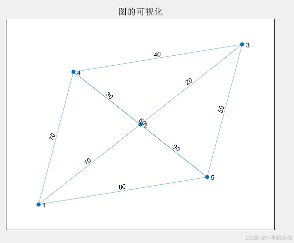

结论

图与网络模型是解决复杂系统问题的重要工具，通过合理的算法和数学模型，可以有效地解决最短路径、最小生成树等问题。利用matlab和python等工具，可以大大简化计算过程，提高工作效率。在实际应用中，图与网络模型广泛用于通信网络建设、物流运输规划等领域，具有重要的现实意义。希望这篇详细的博客总结能够帮助您理解和应用图与网络模型的基本概念、算法及其在实际问题中的应用。