Python实现线性拟合及绘图的示例代码_Python

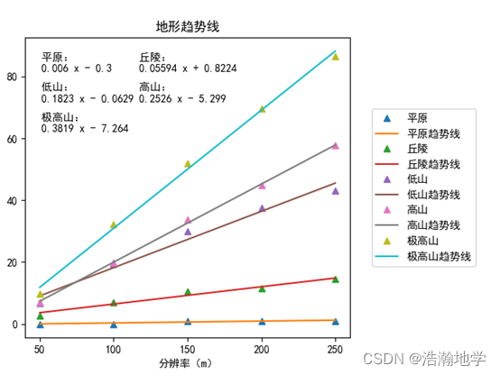
当时的数字地形实验，使用 matplotlib库绘制了一张图表表示不同地形类别在不同分辨率下的rmse值，并分别拟合了一条趋势线。现在来看不足就是地形较多时，需要使用循环更好一点，不然太冗余了。

环境：python 3.9

代码逻辑

导入所需库以及初步设置

# coding=gbk
# -*- coding = utf-8 -*-

import matplotlib.pyplot as plt
import numpy as np
plt.subplots_adjust(left=0.05, right=0.7, top=0.9, bottom=0.1)
plt.rcparams['font.sans-serif'] = ['simhei']

准备数据（这里仅展示部分）

resolutions = [50, 100, 150, 200, 250]
plain = [0, 0, 1, 1, 1]
hill = [2.645751311, 7.071067812, 10.44030651, 11.48912529, 14.4222051]

这里可以改为在excel中读取，尤其是数据多的时候

分别绘制不同数据的趋势线

# 绘制平原趋势线
coefficients_plain = np.polyfit(resolutions, plain, 1)
poly_plain = np.poly1d(coefficients_plain)
plt.plot(resolutions, plain, '^', label="平原")
plt.plot(resolutions, poly_plain(resolutions), label="平原趋势线")

# 绘制丘陵趋势线
coefficients_hill = np.polyfit(resolutions, hill, 1)
poly_hill = np.poly1d(coefficients_hill)
plt.plot(resolutions, hill, '^', label="丘陵")
plt.plot(resolutions, poly_hill(resolutions), label="丘陵趋势线")

使用np.polyfit函数拟合一阶多项式（直线），然后使用np.poly1d构造多项式对象。绘制原始数据点（用’^'标记）和对应的拟合趋势线。

计算指标

# 计算平原趋势线的r值和r方
residuals_plain = plain - poly_plain(resolutions)
ss_residuals_plain = np.sum(residuals_plain**2)
ss_total_plain = np.sum((plain - np.mean(plain))**2)
r_squared_plain = 1 - (ss_residuals_plain / ss_total_plain)
r_plain = np.sqrt(r_squared_plain)

# 计算丘陵趋势线的r值和r方
residuals_hill = hill - poly_hill(resolutions)
ss_residuals_hill = np.sum(residuals_hill**2)
ss_total_hill = np.sum((hill - np.mean(hill))**2)
r_squared_hill = 1 - (ss_residuals_hill / ss_total_hill)
r_hill = np.sqrt(r_squared_hill)

计算得到r方和r值

绘图和打印指标

# 设置图例和标题
plt.legend()
plt.legend(loc='center left', bbox_to_anchor=(1.05, 0.5))
plt.title("地形趋势线")

# 设置坐标轴标题
new_ticks = np.arange(50, 251, 50)
plt.xticks(new_ticks)
plt.xlabel('分辨率（m）')
plt.ylabel('rmse')
formula1 = "平原：{}".format(poly_plain)
plt.text(0.05, 0.95, formula1, transform=plt.gca().transaxes,
         fontsize=10, verticalalignment='top')
formula1 = "丘陵：{}".format(poly_hill)
plt.text(0.35, 0.95, formula1, transform=plt.gca().transaxes,
         fontsize=10, verticalalignment='top')

# 显示图形
plt.figure(figsize=(10, 10))
plt.show()

# 打印
print("平原趋势线公式：", poly_plain)
print("丘陵趋势线公式：", poly_hill)
print("平原趋势线：")
print("r值：", r_plain)
print("r方：", r_squared_plain)
print()
print("丘陵趋势线：")
print("r值：", r_hill)
print("r方：", r_squared_hill)
print()

完整代码

# coding=gbk
# -*- coding = utf-8 -*-

import matplotlib.pyplot as plt
import numpy as np
plt.subplots_adjust(left=0.05, right=0.7, top=0.9, bottom=0.1)
plt.rcparams['font.sans-serif'] = ['simhei']

resolutions = [50, 100, 150, 200, 250]
plain = [0, 0, 1, 1, 1]
hill = [2.645751311, 7.071067812, 10.44030651, 11.48912529, 14.4222051]

# 绘制平原趋势线
coefficients_plain = np.polyfit(resolutions, plain, 1)
poly_plain = np.poly1d(coefficients_plain)
plt.plot(resolutions, plain, '^', label="平原")
plt.plot(resolutions, poly_plain(resolutions), label="平原趋势线")

# 绘制丘陵趋势线
coefficients_hill = np.polyfit(resolutions, hill, 1)
poly_hill = np.poly1d(coefficients_hill)
plt.plot(resolutions, hill, '^', label="丘陵")
plt.plot(resolutions, poly_hill(resolutions), label="丘陵趋势线")

# 计算平原趋势线的r值和r方
residuals_plain = plain - poly_plain(resolutions)
ss_residuals_plain = np.sum(residuals_plain**2)
ss_total_plain = np.sum((plain - np.mean(plain))**2)
r_squared_plain = 1 - (ss_residuals_plain / ss_total_plain)
r_plain = np.sqrt(r_squared_plain)

# 计算丘陵趋势线的r值和r方
residuals_hill = hill - poly_hill(resolutions)
ss_residuals_hill = np.sum(residuals_hill**2)
ss_total_hill = np.sum((hill - np.mean(hill))**2)
r_squared_hill = 1 - (ss_residuals_hill / ss_total_hill)
r_hill = np.sqrt(r_squared_hill)

# 设置图例和标题
plt.legend()
plt.legend(loc='center left', bbox_to_anchor=(1.05, 0.5))
plt.title("地形趋势线")

# 设置坐标轴标题
new_ticks = np.arange(50, 251, 50)
plt.xticks(new_ticks)
plt.xlabel('分辨率（m）')
plt.ylabel('rmse')
formula1 = "平原：{}".format(poly_plain)
plt.text(0.05, 0.95, formula1, transform=plt.gca().transaxes,
         fontsize=10, verticalalignment='top')
formula1 = "丘陵：{}".format(poly_hill)
plt.text(0.35, 0.95, formula1, transform=plt.gca().transaxes,
         fontsize=10, verticalalignment='top')

# 显示图形
plt.figure(figsize=(10, 10))
plt.show()

# 打印
print("平原趋势线公式：", poly_plain)
print("丘陵趋势线公式：", poly_hill)
print("平原趋势线：")
print("r值：", r_plain)
print("r方：", r_squared_plain)
print()
print("丘陵趋势线：")
print("r值：", r_hill)
print("r方：", r_squared_hill)
print()